Differentiation

Partial derivatives

Definition (Partial derivative)

Let \(f:D \subseteq \mathbb{R}^n \to \mathbb{R}\) with \(D\) a neighbourhood of \(a\). For \(j \in \{ 1,\dots,n \}\), the partial derivative of \(f\) at \(a = (a_{1},\dots,a_{n})\) with respect to the \(j\)-th entry is defined as

\[D_{j}f(a) = \lim_{ h \to 0} \frac{f(a_{1},\dots,a_{j-1}, a_{j}+h, a_{j+1},\dots,a_{n}) - f(a)}{h}.\]

Note:

1. If \(y=f(x)\), then \(f'(a) = \lim_{ h \to 0 } \frac{f(a+h)-f(a)}{h}\).
2. We write \(D_{j}f(a) = \frac{\partial f}{\partial x_{j}}(a) = f_{x_{j}}(a)\).
3. The variables \(x_{i} \neq x_{j}\) for every \(i\) are treated as constants.
4. If I define \(g(x_{j}) = f(a_{1},\dots,a_{j-1}, x_{j}, a_{j+1},\dots, a_{n})\), then \(D_{j}f(a) = g'(a_{j})\).
5. Geometrically, for \(n=2\), \(D_{1}f(a,b)\) is the slope at \(x = a\) of the curve obtained by cutting the graph \(z = f(x,y)\) with the plane \(y = b\). The partial derivative only “sees” \(f\) along that line.

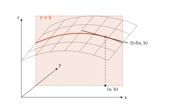
Example

If \(f(x,y,z) = e^{xy^{2}} + \sin(xyz)\) then \(D_{1}f(x,y,z) = e^{xy^{2}}y^{2} + \cos(xyz) \cdot yz\).

Definition (Higher-order partial derivatives)

Given \(f\) such that \(D_{j} f(a)\) exists for every \(j \in \{ 1,\dots n \}\), we define \(D_{ij}f(a) = D_{i} (D_{j} f(a))\). We write \(D_{ij} f(a) = \frac{\partial}{\partial x_i}(\frac{\partial f}{\partial x_{j}})(a) = f_{x_{j}x_{i}}(a)\).

Note:

The notation extends, e.g., \(\frac{\partial^{4} f}{\partial x_{1} \partial x_{2} \partial x_{4} \partial x_{3}}(a)\).

Theorem (Schwarz)

Let \(f:D \subseteq \mathbb{R}^n \to \mathbb{R}\), with \(a \in D\). Suppose that \(f\) is continuous on \(B_{r}(a) \subseteq D\), that \(D_{1}f\), \(D_{2} f\) and \(D_{21} f = D_{2}(D_{1}f)\) exist on \(B_{r}(a)\), and that \(D_{21} f\) is continuous at \(a\). Then \(D_{12} f(a) = D_{1}(D_{2}f)(a)\) exists and \(D_{12}f(a) = D_{21}f(a)\).

Proof: For \(n = 2\), let \(a = (x_{0},y_{0})\) and let \(\varepsilon>0\). By continuity of \(D_{21}f\) at \(a\), there exists \(\delta>0\) such that \([x_{0}-\delta,x_{0}+\delta] \times [y_{0}-\delta,y_{0}+\delta] \subseteq B_{r}(a)\) and \(\lvert D_{21}f(x,y) - D_{21}f(a) \rvert < \varepsilon\) whenever \(\lvert x-x_{0} \rvert<\delta\) and \(\lvert y-y_{0} \rvert < \delta\). Fix \(0<h,k<\delta\) and consider the second difference of \(f\) over the rectangle with vertices \((x_{0},y_{0})\), \((x_{0}+h,y_{0})\), \((x_{0},y_{0}+k)\) and \((x_{0}+h,y_{0}+k)\):

\[\Delta(h,k) = f(x_{0}+h,y_{0}+k) - f(x_{0}+h,y_{0}) - f(x_{0},y_{0}+k) + f(x_{0},y_{0}).\]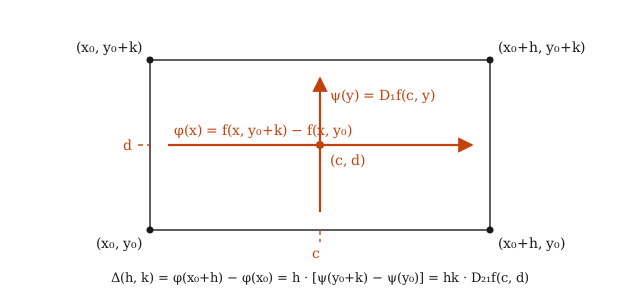

Define \(\phi(x) = f(x, y_{0}+k) - f(x,y_{0})\), so that \(\Delta(h,k) = \phi(x_{0}+h) - \phi(x_{0})\). Since \(D_{1}f\) exists, \(\phi\) is differentiable on \([x_{0},x_{0}+h]\) and, by the mean value theorem, there exists \(c \in (x_{0}, x_{0}+h)\) such that

\[\Delta(h,k) = \phi'(c) \cdot h = h\,(D_{1}f(c, y_{0}+k) - D_{1}f(c,y_{0})).\]

Now define \(\psi(y) = D_{1}f(c,y)\) with \(y \in [y_{0},y_{0}+k]\). Since \(D_{21}f = D_{2}(D_{1}f)\) exists, \(\psi\) is differentiable and, again by the mean value theorem, there exists \(d \in (y_{0},y_{0}+k)\) such that \(\psi(y_{0}+k) - \psi(y_{0}) = \psi'(d) \cdot k = D_{21} f(c,d) \cdot k\). Hence

\[\frac{\Delta(h,k)}{hk} = D_{21} f(c,d), \qquad (c,d) \in (x_{0},x_{0}+h)\times(y_{0},y_{0}+k),\]

and by the choice of \(\delta\),

\[\left\lvert \frac{\Delta(h,k)}{hk} - D_{21}f(a) \right\rvert < \varepsilon \quad \text{for all } 0<h,k<\delta. \tag{1}\]

The key point is that the bound (1) is uniform: it does not depend on where \(c\) and \(d\) landed (which do depend on \(h\) and \(k\)). Fix \(h\) and let \(k \to 0\). Since \(D_{2}f\) exists at \((x_{0}+h,y_{0})\) and at \((x_{0},y_{0})\),

\[\lim_{ k \to 0 } \frac{\Delta(h,k)}{hk} = \frac{1}{h}\left( \lim_{ k \to 0 } \frac{f(x_{0}+h,y_{0}+k) - f(x_{0}+h,y_{0})}{k} - \lim_{ k \to 0 }\frac{f(x_{0},y_{0}+k)-f(x_{0},y_{0})}{k} \right) = \frac{D_{2}f(x_{0}+h,y_{0}) - D_{2}f(x_{0},y_{0})}{h},\]

and passing to the limit in (1) we obtain \(\left\lvert \frac{D_{2}f(x_{0}+h,y_{0}) - D_{2}f(x_{0},y_{0})}{h} - D_{21}f(a) \right\rvert \leq \varepsilon\) for all \(0<h<\delta\) (the case \(h<0\) or \(k<0\) is identical). Since \(\varepsilon\) was arbitrary, this says exactly that the limit as \(h \to 0\) of the difference quotient of \(D_{2}f\) exists and equals \(D_{21}f(a)\); that is,

\[D_{1}(D_{2}f) (x_{0}, y_{0}) = D_{12} f (x_{0},y_{0}) = D_{21} f(x_{0},y_{0}),\]

from which the result follows.

Note

For \(f:\mathbb{R}^{2} \to \mathbb{R}\) of class \(C^{3}\), \(D_{121} f(a,b) = D_{112} f(a,b) = D_{211} f(a,b)\): it suffices to apply the theorem repeatedly. If \(f:\mathbb{R}^{n} \to \mathbb{R}\), the result still holds for each pair of indices \(i \neq j\) (the other variables stay fixed, so it is the case \(n=2\)) and the intuition of the proof is the same. In particular, if \(f \in C^{2}(D)\) then \(D_{ij}f = D_{ji}f\) on \(D\) for all \(i,j\): the order of differentiation does not matter.

Example (without continuity of the mixed partial, the order does matter)

Let

\[f(x,y) = \begin{cases} \frac{xy(x^{2}-y^{2})}{x^{2}+y^{2}} \quad \text{if }(x,y) \neq (0,0) \\ 0 \quad \quad \quad \text{if }(x,y) = (0,0) \end{cases}.\]

For \((x,y) \neq (0,0)\), differentiating the quotient \(\frac{x^{3}y - xy^{3}}{x^{2}+y^{2}}\),

\[D_{1}f(x,y) = \frac{y(x^{4}+4x^{2}y^{2}-y^{4})}{(x^{2}+y^{2})^{2}}, \qquad D_{2}f(x,y) = \frac{x(x^{4}-4x^{2}y^{2}-y^{4})}{(x^{2}+y^{2})^{2}},\]

and since \(f\) vanishes on the axes, \(D_{1}f(0,0) = D_{2}f(0,0) = 0\). Evaluating on the axes: \(D_{1}f(0,y) = \frac{-y^{5}}{y^{4}} = -y\) and \(D_{2}f(x,0) = \frac{x^{5}}{x^{4}} = x\). Therefore

\[D_{21}f(0,0) = \lim_{ k \to 0 } \frac{D_{1}f(0,k) - D_{1}f(0,0)}{k} = \lim_{ k \to 0 } \frac{-k}{k} = -1, \qquad D_{12}f(0,0) = \lim_{ h \to 0 } \frac{D_{2}f(h,0) - D_{2}f(0,0)}{h} = \lim_{ h \to 0 } \frac{h}{h} = 1.\]

The two mixed partials exist at the origin and are different. The hypothesis that fails is the continuity of \(D_{21}f\) at \((0,0)\): in fact \(D_{21}f\) takes values as far apart as \(-1\) and \(1\) in every neighbourhood of the origin.

Theorem (Mean value theorem)

Cf. The Riemann integral (MA0350, MVT in one variable). Let \(f: B_{\delta}(a) \subseteq \mathbb{R}^n \to \mathbb{R}\). Suppose that \(f\) is continuous and that for every \(j \in \{ 1,\dots,n \},\) \(D_{j}(f)\) exists and is continuous. Then, for every \(x \in B_{\delta}(a)\), there exist \(\xi_{1}, \dots \xi_{n} \in B_{\delta}(a)\) such that, if \(x = (x_{1},\dots, x_{n})\) and \(a = (a_{1}, \dots, a_{n})\), then

\[f(x) - f(a)= \sum_{j=1}^{n} D_{j} f(\xi_{j}) (x_{j} - a_{j}).\]

Proof: For \(n=2\), note that

\[f(x) - f(a) = f(x_{1},x_{2}) - f(a_{1}, x_{2}) + f(a_{1},x_{2}) - f(a_{1},a_{2}).\]

Let \(g(t) = f(t,x_{2})\) and \(h(t) = f(a_{1},t)\). Then

\[\begin{aligned} \implies f(x)-f(a) &= g(x_{1}) - g(a_{1}) + h(x_{2}) - h(a_{2}) \\ &\underset{TVM}{=} g'(t_{1}) (x_{1}-a_{1}) + h'(t_{2})(x_{2}-a_{2}) \\ &= D_{1}f(\underbrace{ t_{1},x_{2} }_{ \xi_{1} })(x_{1}-a_{1}) + D_{2} f(\underbrace{ a_{1}, t_{2} }_{ \xi_{2} })(x_{2}-a_{2}), \end{aligned}\]

with \(t_{i}\) between \(x_{i}\) and \(a_{i}\). The points \(\xi_{1} = (t_{1},x_{2})\) and \(\xi_{2} = (a_{1},t_{2})\) lie in the ball because \(\lVert \xi_{1}-a \rVert^{2} = (t_{1}-a_{1})^{2} + (x_{2}-a_{2})^{2} \leq \lVert x-a \rVert^{2}\), and similarly for \(\xi_{2}\). The argument is analogous for \(n>2\): one passes from \(a\) to \(x\) changing one coordinate at a time.

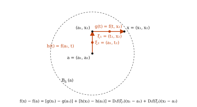
Note

The theorem is for scalar functions. For \(f:\mathbb{R}^n \to \mathbb{R}^{m}\) with \(m>1\) it applies componentwise, but the intermediate points \(\xi\) change from one component to another, and in general there is no single \(\xi\) that works for all of them. For instance, \(\gamma(t) = (\cos t, \sin t)\) satisfies \(\gamma(2\pi) - \gamma(0) = (0,0)\), but \(\gamma'(t) = (-\sin t, \cos t) \neq (0,0)\) for every \(t\), so there is no \(\xi\) with \(\gamma(2\pi)-\gamma(0) = \gamma'(\xi)\cdot 2\pi\). What does survive is the mean value inequality: if \(f \in C^{1}\) on a convex open set containing \(a\) and \(x\), then \(\lVert f(x) - f(a) \rVert \leq \sup_{\xi} \lVert J_{f}(\xi) \rVert \, \lVert x-a \rVert\), with the supremum taken over the segment.

Example

Consider

\[f(x,y) = \begin{cases} \frac{xy}{x^{2}+y^{2}} \quad \text{if }(x,y) \neq (0,0) \\ 0 \quad \quad \quad \text{if }(x,y) = (0,0) \end{cases}.\]

Note that

1. \(f\) is not continuous at \((0,0)\): on the line \(y = x\) we have \(f(x,x) = \frac{x^{2}}{2x^{2}} = \frac{1}{2}\) for every \(x \neq 0\), whereas \(f(0,0) = 0\).
2. \(\frac{\partial f}{\partial x} (0,0) = \lim_{ h \to 0 } \frac{f(h,0)-f(0,0)}{h} = \lim_{ h \to 0 } \frac{\frac{0 \cdot h}{h^{2}+0^{2}} - 0}{h} = 0\).
3. Now, if \((a,b) \neq (0,0)\), then

\[\frac{\partial f}{\partial x}(a,b) = \frac{(x^{2}+y^{2})y - xy \cdot 2x}{(x^{2}+y^{2})^{2}} \biggr\rvert_{(x,y)=(a,b)} = \frac{b(b^{2}-a^{2})}{(a^{2}+b^{2})^{2}}.\]

So

\[\frac{\partial f(x,y)}{\partial x} = \begin{cases} \frac{y(y^{2}-x^{2})}{(x^{2}+y^{2})^{2}} \quad \text{if }(x,y) \neq (0,0) \\ 0 \quad \quad \quad \text{if }(x,y) = (0,0) \end{cases}\]

and by symmetry \(\frac{\partial f}{\partial y}(x,y) = \frac{x(x^{2}-y^{2})}{(x^{2}+y^{2})^{2}}\) away from the origin, with \(\frac{\partial f}{\partial y}(0,0) = 0\). Thus both partial derivatives exist on all of \(\mathbb{R}^{2}\) and yet \(f\) is not continuous at \((0,0)\): in several variables, the existence of the partial derivatives does not imply continuity. Note also that \(\frac{\partial f}{\partial x}\) is not continuous at \((0,0)\); it is not even bounded, since \(\frac{\partial f}{\partial x}(0,y) = \frac{y^{3}}{y^{4}} = \frac{1}{y} \to \infty\) as \(y \to 0^{+}\). This is consistent with the next theorem: the continuity of the partials is exactly what is missing.

Theorem (Partial derivatives and continuity)

Let \(f:D\subseteq \mathbb{R}^n \to \mathbb{R}\) be such that \(\frac{\partial f}{\partial x_{i}}(x)\) exists and is continuous on \(D\) (open) for every \(i \in \{ 1,\dots,n \}\). Then \(f\) is continuous on \(D\).

Proof: Let \(a \in D, \varepsilon>0\). Then there exists \(r>0\) such that \(B:=\bar{B}_{r}(a) \subseteq D\). Since \(B\) is compact and the \(\frac{\partial f}{\partial x_{i}}(x)\) are continuous, there exist \(M_{i} > 0\) for every \(i \in \{ 1,\dots,n \}\) such that \(\left\lvert \frac{\partial f}{\partial x_{j}} (x) \right\rvert \leq M_{j}\) for every \(x \in B\). Let \(M = \max \{ M_{1}, \dots, M_{n} \}>0\). Take \(\delta < \min \left\{ \frac{\varepsilon}{Mn},r \right\}\). Suppose that \(\lVert x-a \rVert<\delta\), so that \(x \in B\) and \(\lvert x_{j}-a_{j} \rvert < \delta\) for every \(j\). Then, by the mean value theorem, \(f(x)-f(a) = \sum_{j=1}^{n} \frac{\partial f}{\partial x_{j}}(\xi_{j})(x_{j}-a_{j})\), with \(\xi_{1}, \xi_{2},\dots,\xi_{n} \in B\). Then

\[\begin{aligned} \lvert f(x)-f(a) \rvert &\leq \sum_{j=1}^{n} \left\lvert \frac{\partial f}{\partial x_{j}}(\xi_{j}) \right\rvert \lvert x_{j}-a_{j} \rvert \\ &\leq \sum_{j=1}^{n} M\delta = nM\delta < \varepsilon \end{aligned}\]

Theorem (Relative extrema and partial derivatives)

Given \(f:D \subseteq \mathbb{R}^n \to \mathbb{R}\), suppose that \(f\) attains a relative extremum at \(c \in D^{\circ}\). If \(\frac{\partial f}{\partial x_{j}}(c)\) exists, then \(\frac{\partial f}{\partial x_{j}}(c) = 0\).

Proof: Define \(g(x) = f(c_{1},c_{2},\dots,c_{j-1},x,c_{j+1},\dots,c_{n})\) with \(c = (c_{1},\dots,c_{n})\), defined on an open interval around \(c_{j}\) (since \(c\) is an interior point). Then \(g'(c_{j}) = \frac{\partial f}{\partial x_{j}}(c)\). Since \(g\) has a relative extremum at \(c_{j}\), by the one-variable result \(g'(c_{j}) = \frac{\partial f}{\partial x_{j}}(c) = 0\).

Note

Let \(f:\mathbb{R} \to \mathbb{R}\). Its derivative is \(f'(a) = \lim_{ x \to a } \frac{f(x)-f(a)}{x-a} = \lim_{ h \to 0 }\frac{f(a+h)-f(a)}{h}\). This is the notion of differentiability in one variable; the previous example shows that having partial derivatives is too weak a condition in several variables (it does not even give continuity). What is the right notion of differentiability?

Differentiability

Note

In one dimension, \(f'(a)\) exists if and only if \(\lim_{ h \to 0 } \frac{f(a+h)-f(a)-f'(a)h}{h} = 0\).

Definition (Differentiability)

Given \(f:D \subseteq \mathbb{R}^n\to \mathbb{R}^{m}\), with \(D\) a neighbourhood of \(a\). We say that \(f\) is differentiable at \(a\) if there exists a linear transformation \(T:\mathbb{R}^n\to \mathbb{R}^{m}\) such that

\[\lim_{ \vec{h} \to 0 } \frac{\lVert f(a+\vec{h}) - f(a) - T(\vec{h}) \rVert_{m}}{\lVert \vec{h} \rVert_{n}} = 0\]

Notes

1. \(\frac{\partial f}{\partial x_{j}}(c) = \lim_{ h \to 0 } \frac{f(c+h e_{j})-f(c)}{h}\), where \(e_{j}\) is the \(j\)-th standard basis vector.
2. If the function is differentiable at \(a\), we write \(D_{f}(a)=T\)
3. Evaluating \(D_{f}\) is written \(D_{f}(a)(x) = T(x)\).
4. For \(m = 1\), the definition says that \(f(a+h) = f(a) + T(h) + r(h)\) with \(\frac{r(h)}{\lVert h \rVert} \to 0\): the graph of the affine function \(x \mapsto f(a) + T(x-a)\) is the tangent plane to the graph of \(f\) at \((a,f(a))\), and the error of approximating \(f\) by that plane is small even compared with \(\lVert h \rVert\). That is the difference from merely having partial derivatives: the partials control the error along \(n\) lines; differentiability controls it in all directions at once.

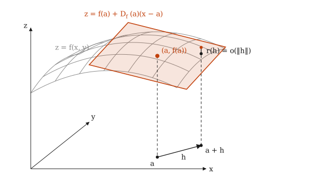
Example

Consider \(f:\mathbb{R}^n\to \mathbb{R}^{m}\), with \(f(x) = c \in \mathbb{R}^{m}\). If \(T(x) = 0\), then \(D_{f}(a) = 0\), since

\[\lim_{ h \to 0} \frac{\lVert c-c-0 \rVert }{\lVert h \rVert } = 0\]

Example

If \(f:\mathbb{R}\to \mathbb{R}\) is differentiable at \(a\), then \(D_{f}(a)(h) = f'(a) h\). The differential can be used to make approximations, for instance Taylor’s: \(f(a+h) \approx f(a) + hf'(a)\).

Example

Consider \(f:\mathbb{R}^{2}\to \mathbb{R}\) with \(f(x,y) = x^{2}+3y\). What is \(D_{f}(a,b)\)? Let \((h,k)\) be the increment in the limit. Note that

\[\begin{aligned} & \lim_{ (h,k) \to (0,0) } \frac{\lvert (a+h)^{2}+3(b+k) - a^{2}-3b-T(h,k) \rvert }{\lVert (h,k)\rVert } \\ &= \lim_{ (h,k) \to (0,0) } \frac{\lvert 2ah+h^{2}+3k-T(h,k) \rvert }{ \sqrt{h^{2}+k^{2}}}=L \end{aligned}\]

Take \(T(h,k) = 2ah + 3k\). Clearly \(T\) is linear and moreover, if \((h,k) \longrightarrow (0,0)\) then \(T(h,k)\longrightarrow 0\). So

\[L=\lim_{ (h,k) \to (0,0)} \frac{h^{2}}{\sqrt{ h^{2}+k^{2} }} = 0\]

since

\[0 \leq \frac{h^{2}}{\sqrt{ h^{2}+k^{2} }} \leq \frac{h^{2}}{\sqrt{ h^{2} }} = \lvert h \rvert \underset{(h,k) \rightarrow (0,0)}{\longrightarrow} 0,\]

and therefore \(D_{f}(a,b)(h,k) = 2ah+3k =\begin{pmatrix}2a & 3\end{pmatrix} \begin{pmatrix}h \\ k\end{pmatrix}\).

Example

Let \(f(x,y) = xy\). At \((a,b)\), \(f(a+h,b+k) - f(a,b) = (a+h)(b+k) - ab = bh + ak + hk\). The linear candidate is the degree-1 part of the increment, \(T(h,k) = bh + ak\), and the remainder is \(hk\). Since \(\lvert hk \rvert \leq \frac{h^{2}+k^{2}}{2}\),

\[\frac{\lvert hk \rvert}{\sqrt{ h^{2}+k^{2} }} \leq \frac{\sqrt{ h^{2}+k^{2} }}{2} \underset{(h,k) \rightarrow (0,0)}{\longrightarrow} 0,\]

so \(f\) is differentiable at \((a,b)\) with \(D_{f}(a,b)(h,k) = bh + ak\) (in agreement with \(\nabla f(a,b) = (b,a)\), as we shall see). Recipe for polynomials: expand \(f(a+h)\), keep the part that is linear in \(h\), and check that whatever is left over, divided by \(\lVert h \rVert\), tends to zero.

### Theorem (Uniqueness of the differential) If \(f\) is differentiable at \(a\), its differential is unique.

Proof: Suppose there exist linear \(T, S: \mathbb{R}^n \to \mathbb{R}^{m}\) both satisfying the definition. Then

\[\begin{aligned} \frac{\lVert T(h)-S(h) \rVert }{\lVert h \rVert } \leq \frac{\lVert T(h) - f(a+h) + f(a) \rVert }{\lVert h \rVert } + \frac{\lVert f(a+h) - f(a) - S(h) \rVert }{\lVert h \rVert } \underset{h \rightarrow 0}{\longrightarrow} 0. \end{aligned}\]

I need \(T(x) = S(x) \quad \forall x \in \mathbb{R}^n\). So, if \(x \in \mathbb{R}^n\setminus \{ 0 \}\), \(t \in \mathbb{R}\), take \(h = tx\). Then

\[0 = \lim_{ t \to 0 } \frac{\lVert T(tx) - S(tx) \rVert }{\lVert tx \rVert } = \lim_{ t \to 0 } \frac{\lVert T(x) - S(x) \rVert }{\lVert x \rVert } = \frac{\lVert T(x) - S(x) \rVert }{\lVert x \rVert },\]

so \(T(x) = S(x)\) for every \(x \in \mathbb{R}^n\setminus \{ 0 \}\) (equality at zero holds trivially since they are linear transformations), and therefore \(S = T\).

Theorem (Differentiability implies continuity)

If \(f\) is differentiable at \(a\), then \(f\) is continuous at \(a\).

Proof: Let \(\varepsilon>0\). By differentiability there exists \(\delta_{1}>0\) such that if \(\lVert h \rVert < \delta_{1}\) then

\[\frac{\lVert f(a+h) - f(a) - D_{f}(a)(h) \rVert }{\lVert h \rVert} < \varepsilon. \ \tag{1}\]

Since \(D_{f}(a)\) is linear, it is continuous. There exists \(\delta_{2}>0\) such that \(\lVert x-a \rVert<\delta_{2} \implies \lVert D_{f}(a)(x) - D_{f}(a)(a) \rVert < \frac{\varepsilon}{2}.\) Take \(\delta = \min \left\{ \delta_{1}, \delta_{2}, \frac{1}{2} \right\}\). Suppose that \(\lVert x-a \rVert < \delta\). Then

\[\begin{aligned} \lVert f(x)-f(a) \rVert &\leq \lVert f(x) - f(a) - D_{f}(a)(x-a) \rVert + \lVert D_{f}(a)(x-a) \rVert \\ &\leq \varepsilon \lVert x-a \rVert + \frac{\varepsilon}{2} \quad \quad \text{taking } h =x-a \text{ in (1)}\\ &< \varepsilon \delta + \frac{\varepsilon}{2} \leq \varepsilon. \end{aligned}\]

We conclude that \(f\) is continuous at \(a\).

Definition (Directional derivative)

Given \(f:\mathbb{R}^n\to \mathbb{R}\), \(\vec{u} \in \mathbb{R}^n\), \(\lVert \vec{u} \rVert = 1\), the directional derivative along \(\vec{u}\) is defined as

\[D_{\vec{u}}f(a) = \lim_{ h \to 0 } \frac{f(a+h \vec{u}) - f(a)}{h}.\]

Note

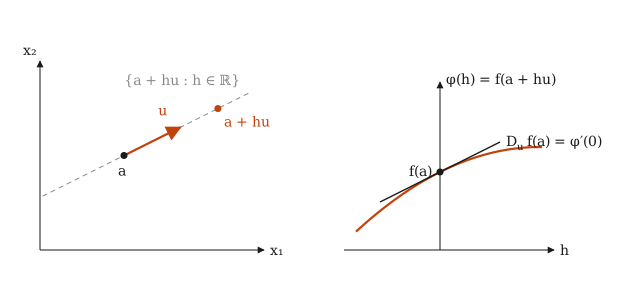
If \(\vec{u} = e_{j}\), then \(D_{\vec{u}}f(a) = \frac{\partial f(a)}{\partial x_{j}}\), since \(a+h \vec{u} = a+h e_{j}\). The directional derivative measures the rate of change of \(f\) as one leaves \(a\) along the line \(\{ a + h\vec{u} : h \in \mathbb{R} \}\): it is the derivative at \(h = 0\) of the one-variable function \(\varphi(h) = f(a+h\vec{u})\). We require \(\lVert \vec{u} \rVert = 1\) so that \(h\) measures the distance travelled; otherwise the same definition gives \(D_{\lambda \vec{u}}f(a) = \lambda D_{\vec{u}}f(a)\).

Theorem (Differentiability and directional derivatives)

Let \(f:D \subseteq \mathbb{R}^n\to \mathbb{R}\), \(a \in D\) open. If \(f\) is differentiable at \(a\), then \(D_{\vec{u}}f(a)\) exists for every unit vector \(\vec{u} \in \mathbb{R}^n\), and \(D_{\vec{u}}f(a) = D_{f}(a)(u)\).

Proof: Note that

\[\begin{aligned} D_{\vec{u}}f(a) &= \lim_{ h \to 0 }\underbrace{ \frac{f(a+h \vec{u}) - f(a)-D_{f}(a)(hu)}{h} }_{ \longrightarrow 0 } + \frac{D_{f}(a)(\cancel{ h }u)}{\cancel{ h }} \\ &= D_{f}(a)(u), \end{aligned}\]

from which the result follows.

Corollary

Under the same hypothesis, \(\frac{\partial f}{\partial x_{1}}, \dots, \frac{\partial f}{\partial x_{n}}\) exist and \(D_{f}(a)(y) = \sum_{i=1}^{n} \frac{\partial f(a)}{\partial x_{i}} y_{i}\) with \(y = (y_{1}, \dots, y_{n})\).

Proof: The partial derivatives exist by the previous theorem, taking \(u\) to be each of the standard basis vectors. Moreover,

\[\begin{aligned} D_{f}(a)(y) &= D_{f}(a)\left( \sum_{i=1}^{n} e_{i} y_{i} \right) \\ &= \sum_{i=1}^{n} y_{i} D_{f}(a)(e_{i}) \\ &= \sum_{i=1}^{n} y_{i} \frac{\partial f(a)}{\partial x_{i}}. \end{aligned}\]

Note

In vector notation,

\[D_{f}(a)(y) = \underbrace{ \begin{pmatrix} \frac{ \partial f(a) }{ \partial x_{1}} \\ \vdots \\ \frac{ \partial f(a) }{ \partial x_{n} } \end{pmatrix} }_{ \text{gradient of } f \text{ at } a \text{: }\nabla f(a)} \cdot \quad \begin{pmatrix} y_{1} \\ \vdots \\ y_{n} \end{pmatrix} \implies D_{f}(a)(y) = \nabla f(a) \cdot y.\]

Example

Consider \(f:\mathbb{R}^{3} \to \mathbb{R}\) with \(f(x,y,z)= x^{2}+yz\). Then

\[\nabla f (x,y,z) = \begin{bmatrix} \frac{ \partial f }{ \partial x }(x,y,z) \\ \frac{ \partial f }{ \partial y }(x,y,z) \\ \frac{ \partial f }{ \partial z }(x,y,z) \end{bmatrix} = \begin{bmatrix} 2x \\ z \\ y \end{bmatrix}.\]

If \(a = (1,-1,0)\), then \(\nabla f(a) =\begin{bmatrix}2 & 0 & -1\end{bmatrix}^{T}\) and so

\[D_{f}(a)(x,y,z) = \begin{bmatrix} 2 \\ 0 \\ -1 \end{bmatrix} \cdot \begin{bmatrix} x \\ y \\ z \end{bmatrix} = 2x-z.\]

Example (continuous with partials, yet not differentiable)

Let \(f(x,y) = \sqrt{ \lvert xy \rvert }\). It is continuous on \(\mathbb{R}^{2}\) and vanishes on the axes, so \(D_{1}f(0,0) = \lim_{ h \to 0 }\frac{f(h,0)-f(0,0)}{h} = 0\) and \(D_{2}f(0,0) = 0\). If \(f\) were differentiable at \((0,0)\), by the corollary we would have \(D_{f}(0,0) = 0\) and every directional derivative would be zero. But for \(\vec{u} = \left( \frac{1}{\sqrt{ 2 }}, \frac{1}{\sqrt{ 2 }} \right)\),

\[\frac{f(h\vec{u}) - f(0,0)}{h} = \frac{\sqrt{ h^{2}/2 }}{h} = \frac{\lvert h \rvert}{\sqrt{ 2 }\,h},\]

which equals \(\frac{1}{\sqrt{ 2 }}\) for \(h>0\) and \(-\frac{1}{\sqrt{ 2 }}\) for \(h<0\): the limit does not exist. Hence \(f\) is not differentiable at \((0,0)\) (it does not even have a directional derivative in that direction). Having partials does not imply being differentiable, not even for a continuous function.

Example (all directional derivatives exist, yet not differentiable)

Let

\[f(x,y) = \begin{cases} \frac{x^{2}y}{x^{2}+y^{2}} \quad \text{if }(x,y) \neq (0,0) \\ 0 \quad \quad \quad \text{if }(x,y) = (0,0) \end{cases}.\]

It is continuous at the origin, since \(\lvert f(x,y) \rvert \leq \frac{x^{2}\lvert y \rvert}{x^{2}+y^{2}} \leq \lvert y \rvert\). For a unit vector \(\vec{u} = (u_{1},u_{2})\), since \(f\) is homogeneous of degree 1 (that is, \(f(hx,hy) = h f(x,y)\)),

\[D_{\vec{u}}f(0,0) = \lim_{ h \to 0 } \frac{f(hu_{1},hu_{2})}{h} = \lim_{ h \to 0 } \frac{h\,f(u_{1},u_{2})}{h} = f(u_{1},u_{2}) = u_{1}^{2}u_{2}.\]

So all directional derivatives exist at \((0,0)\); in particular \(D_{1}f(0,0) = D_{2}f(0,0) = 0\). But if \(f\) were differentiable, the theorem would give \(D_{\vec{u}}f(0,0) = \nabla f(0,0) \cdot \vec{u} = 0\) for every \(\vec{u}\), whereas \(u_{1}^{2}u_{2} \neq 0\) in general (e.g. \(\vec{u} = \frac{(1,1)}{\sqrt{ 2 }}\) gives \(\frac{1}{2\sqrt{ 2 }}\)). The obstruction is that \(\vec{u} \mapsto D_{\vec{u}}f(0,0)\) is not linear in \(\vec{u}\), whereas for a differentiable function it always is (\(= D_{f}(a)(\vec{u})\)).

Note (summary of implications at a point \(a\))

\[f \in C^{1} \text{ near } a \implies f \text{ differentiable at } a \implies \begin{cases} f \text{ continuous at } a, \\ \text{all } D_{\vec{u}}f(a) \text{ exist and } \vec{u} \mapsto D_{\vec{u}}f(a) \text{ is linear} \end{cases} \implies \text{the partials exist at } a,\]

and none of the arrows can be reversed: the examples of this section and of the next one are the counterexamples (the first implication is proved further below).

Theorem (Differentiability componentwise)

Let \(f:\mathbb{R}^n \to \mathbb{R}^{m}\), \(f =\begin{pmatrix}f_{1} \\ \vdots \\ f_{m}\end{pmatrix}\), \(f_{j}:\mathbb{R}^n\to \mathbb{R}\). Then \(f\) is differentiable at \(a\) if and only if \(f_{j}\) is differentiable at \(a\) for every \(j \in \{ 1,\dots ,m \}\). Moreover,

\[D_{f}(a) = \begin{bmatrix} D_{f_{1}}(a) \\ \vdots \\ D_{f_{m}}(a) \end{bmatrix}.\]

Proof: We know that for every \(x \in \mathbb{R}^{m}\) and every \(j \in \{ 1,\dots,m \}\), \(\lvert x_{j} \rvert \leq \lVert x \rVert \leq \sum_{j=1}^{m} \lvert x_{j} \rvert\). If \(T = (T_{1},\dots,T_{m})\) is linear (each \(T_{j}:\mathbb{R}^n\to \mathbb{R}\) linear), applying this to \(x = f(a+h)-f(a)-T(h)\) we have that

\[\begin{aligned} 0 \leq \frac{\lvert f_{j}(a+h) - f_{j}(a) - T_{j}(h) \rvert }{\lVert h \rVert } &\leq \frac{\lVert f(a+h) -f(a) - T(h) \rVert }{\lVert h \rVert } \\ &\leq \sum_{j=1}^{m} \frac{\lvert f_{j}(a+h) -f_{j}(a) - T_{j}(h)\rvert}{\lVert h \rVert }. \end{aligned}\]

(\(\implies\)): If \(f\) is differentiable at \(a\) with \(D_{f}(a) = T\), the middle term tends to zero, and by the left-hand inequality so does each quotient \(\frac{\lvert f_{j}(a+h) - f_{j}(a) - T_{j}(h) \rvert }{\lVert h \rVert }\); thus \(f_{j}\) is differentiable at \(a\) with \(D_{f_{j}}(a) = T_{j}\).

(\(\impliedby\)): If each \(f_{j}\) is differentiable at \(a\), take \(T_{j} = D_{f_{j}}(a)\) and \(T = (T_{1},\dots,T_{m})\). Each summand on the right tends to zero, hence so does the middle term, and \(f\) is differentiable at \(a\) with \(D_{f}(a) = T\).

Definition (Jacobian matrix)

Let \(f\) be differentiable at \(a\). Since \(D_{f}(a):\mathbb{R}^n \to \mathbb{R}^{m}\), define \(J_{f}(a)\) (the Jacobian matrix of \(f\) at \(a\)) to be the matrix associated with \(D_{f}(a)\) in the standard bases.

Corollary

If \(f:\mathbb{R}^n\to \mathbb{R}^{m}\), \(f = \begin{pmatrix}f_{1} & \dots & f_{m}\end{pmatrix}^{T}\) is differentiable at \(a\) then \(\frac{ \partial f_{i}(a) }{ \partial x_{j} }\) exists for all \(j \in \{ 1,\dots n \}\), \(i \in \{ 1,\dots,m \}\). Moreover, \([J_{f}(a)]_{ij} = \frac{ \partial f_{i}(a) }{ \partial x_{j} }\). That is

\[J_{f}(a) = \begin{bmatrix} \frac{ \partial f_{1}(a) }{ \partial x_{1} } & \frac{ \partial f_{1}(a) }{ \partial x_{2} } & \dots & \frac{ \partial f_{1}(a) }{ \partial x_{n} } \\ \frac{ \partial f_{2}(a) }{ \partial x_{1} } & \frac{ \partial f_{2}(a) }{ \partial x_{2} } & \dots & \frac{ \partial f_{2}(a) }{ \partial x_{n} } \\ \vdots & \vdots & \ddots & \vdots \\ \frac{ \partial f_{m}(a) }{ \partial x_{1} } & \frac{ \partial f_{m}(a) }{ \partial x_{2} } & \dots & \frac{ \partial f_{m}(a) }{ \partial x_{n} } \end{bmatrix}_{m \times n}\]

Example

Consider \(f(x,y,z) = \begin{pmatrix}x^{2}\sin y - z \\ e^{xy} + zx\end{pmatrix}\). Then

\[J_{f}(x,y,z) = \begin{bmatrix} 2x\sin y & x^{2}\cos y & -1 \\ y e^{xy}+z & xe^{xy} & x \end{bmatrix}.\]

If \((a,b,c) = (1,0,\pi)\),

\[\begin{aligned} \implies J_{f}(a,b,c) &= \begin{bmatrix} 0 & 1 & -1 \\ \pi & 1 & 1 \end{bmatrix} \\ \implies D_{f}(a,b,c)(x,y,z) &= \begin{bmatrix} 0 & 1 & -1 \\ \pi & 1 & 1 \end{bmatrix} \begin{bmatrix} x \\ y \\ z \end{bmatrix} = \begin{bmatrix} y-z \\ \pi x+y+z \end{bmatrix}. \end{aligned}\]

Theorem (Jacobian and gradient)

Let \(f:A\subseteq \mathbb{R}^n \to \mathbb{R}\) with \(A\) open. Suppose that \(f\) is continuously differentiable at \(a\); that is, the first-order partial derivatives of \(f\) exist in a neighbourhood of \(a\) and are continuous at \(a\). Then \(f\) is differentiable at \(a\) and \(J_{f}(a) = \nabla f(a)^{T}\).

Proof: Let \(\varepsilon>0\). By continuity there exist \(\delta_{1},\dots,\delta_{n}\) such that for every \(1\leq j\leq n\), if \(\lVert x-a \rVert <\delta_{j}\) then \(\left\lVert \frac{ \partial f }{ \partial x_{j} }(x) - \frac{ \partial f }{ \partial x_{j} }(a) \right\rVert < \frac{\varepsilon}{n}\). Let \(T:\mathbb{R}^n\to \mathbb{R}\) be a linear transformation with \(T(x_{1},\dots,x_{n}) = \sum_{i=1}^{n} \frac{ \partial f }{ \partial x_{i} }(a) \cdot x_{i}\). Take \(\delta = \min\{ \delta_{1},\dots,\delta_{n} \}\) (shrinking it if necessary so that the partials exist on \(B_{\delta}(a)\)) and let \(h = (h_{1},\dots, h_{n})\) with \(0<\lVert h \rVert < \delta\). By the mean value theorem, there exist \(\xi_{1}, \dots, \xi_{n} \in B_{\delta}(a)\) such that

\[f(a+h)-f(a) = \sum_{i=1}^{n} \frac{ \partial f }{ \partial x_{i} }(\xi_{i}) \cdot h_{i}.\]

So, using this expression in the definition of differentiability, and since \(\lVert \xi_{i} - a \rVert < \delta\):

\[\begin{aligned} \frac{\lvert f(a+h) - f(a) - T(h) \rvert }{\lVert h \rVert } &= \frac{1}{\lVert h \rVert } \left\lvert \sum_{i=1}^{n} \left( \frac{ \partial f }{ \partial x_{i} }(\xi_{i}) - \frac{ \partial f }{ \partial x_{i} }(a) \right) h_{i} \right\rvert \\ &\leq \sum_{i=1}^{n} \left\lvert \frac{ \partial f }{ \partial x_{i} }(\xi_{i}) - \frac{ \partial f }{ \partial x_{i} }(a) \right\rvert \underbrace{ \frac{\lvert h_{i} \rvert }{\lVert h \rVert } }_{ \leq 1 } < \sum_{i=1}^{n} \frac{\varepsilon}{n} = \varepsilon, \end{aligned}\]

from which we conclude that \(D_{f}(a) = T\).

Theorem (Jacobian and gradients for functions into \(\mathbb{R}^{m}\))

Let \(f:A \subseteq \mathbb{R}^n \to \mathbb{R}^{m}\) with \(A\) open and \(a \in A\). Suppose that \(f\) is continuously differentiable at \(a\). Then \(f\) is differentiable at \(a\) and \(J_{f}(a) = [\nabla f_{1}(a), \nabla f_{2}(a),\dots, \nabla f_{m}(a)]^{T}\); that is, row \(j\) of \(J_{f}(a)\) is \(\nabla f_{j}(a)^{T}\).

Proof: By hypothesis, for all \(1 \leq i \leq n\), \(1 \leq j \leq m\), \(D_{i} f_{j}(x)\) exist near \(a\) and are continuous at \(a\). By the previous theorem, \(f_{j}\) is differentiable at \(a\) with \(J_{f_{j}}(a) = \nabla f_{j}(a)^{T}\). Then, since \(f_{j}\) is differentiable at \(a\) for every \(j\), by the componentwise differentiability theorem \(f = (f_{1},\dots,f_{m})\) is differentiable at \(a\) and the rows of \(J_{f}(a)\) are the \(J_{f_{j}}(a)\).

Definition (Classes of functions)

We say that \(f:D \subseteq \mathbb{R}^n \to \mathbb{R}^{m}\) (\(D\) open) is of class \(C^{k}\) (\(f \in C^{k}(D)\)) if all its partial derivatives of order at most \(k\) exist and are continuous on \(D\). By the previous theorem, \(f \in C^{1}(D)\) implies that \(f\) is differentiable at every point of \(D\); the converse is false (see the example below). Similarly, we say that \(f \in C^{\infty}(D)\) if for every \(k \in \mathbb{N}\), \(f \in C^{k}(D)\). If \(f:D\to B\), we write the definition as \(f \in C^{k}(D,B)\).

Example (differentiable but not \(C^{1}\))

Let \(f(x,y) = (x^{2}+y^{2})\sin\left( \frac{1}{\sqrt{ x^{2}+y^{2} }} \right)\) for \((x,y) \neq (0,0)\) and \(f(0,0) = 0\). With \(T = 0\),

\[\frac{\lvert f(h,k) - f(0,0) - 0 \rvert}{\sqrt{ h^{2}+k^{2} }} = \sqrt{ h^{2}+k^{2} }\,\left\lvert \sin\left( \frac{1}{\sqrt{ h^{2}+k^{2} }} \right) \right\rvert \leq \sqrt{ h^{2}+k^{2} } \underset{(h,k) \rightarrow (0,0)}{\longrightarrow} 0,\]

so \(f\) is differentiable at \((0,0)\) with \(D_{f}(0,0) = 0\). However, for \((x,y) \neq (0,0)\), writing \(\rho = \sqrt{ x^{2}+y^{2} }\) and using \(\frac{ \partial \rho }{ \partial x } = \frac{x}{\rho}\),

\[D_{1}f(x,y) = 2x\sin\left( \frac{1}{\rho} \right) - \frac{x}{\rho}\cos\left( \frac{1}{\rho} \right),\]

and on the \(x\)-axis (\(y = 0\), \(x>0\)) this is \(2x\sin\left( \frac{1}{x} \right) - \cos\left( \frac{1}{x} \right)\), which has no limit as \(x \to 0^{+}\). Hence \(D_{1}f\) is not continuous at \((0,0)\) and \(f \notin C^{1}\) on any neighbourhood of the origin: differentiable does not imply \(C^{1}\).

Theorem (Zero gradient)

Let \(f \in C^{1}(D, \mathbb{R}^{m})\) with \(D \subseteq \mathbb{R}^{n}\) open and connected. If \(J_{f}(x) = 0\) for every \(x \in D\) (for \(m=1\): \(\nabla f(x) = 0\)), then \(f\) is constant on \(D\).

Proof: It is enough to prove it for \(m =1\) (apply it to each component). Let \(a \in D\). Since \(D\) is open, there exists \(\delta > 0\) such that \(B_{\delta}(a) \subseteq D\). Let \(x \in B_{\delta}(a)\). By the MVT, there exist \(\xi_{1},\dots,\xi_{n} \in B_{\delta}(a)\) such that \(f(x)-f(a) = \sum_{j=1}^{n} \underbrace{ \frac{ \partial f }{ \partial x_{j} }(\xi_{j}) }_{ =0 } \cdot (x_{j}-a_{j}) = 0\). Hence \(f(x) = f(a)\) for every \(x \in B_{\delta}(a)\): \(f\) is locally constant.

Now let \(A = \{ x \in D:f(x) = f(a) \}\). Note that \(A \neq \emptyset\) since \(a \in A\). Let us see that \(A\) is open: given \(y \in A\), by the above (applied at \(y\)) there exists \(\delta_{y} > 0\) such that \(f(x) = f(y) = f(a)\) for every \(x \in B_{\delta_{y}}(y)\), that is, \(B_{\delta_{y}}(y) \subseteq A\). On the other hand, the set \(B=\{ x \in D: f(x)\neq f(a) \} = f^{-1}[(-\infty,f(a)) \cup(f(a), \infty)]\) is open, being the preimage of an open set under a continuous function defined on the open set \(D\). Since \(D = A \cup B\) with \(A \cap B = \emptyset\), \(A\) and \(B\) open, and \(D\) connected, one of the two is empty. Since \(A \neq \emptyset\), it follows that \(B = \emptyset\). Hence \(A = D\), and therefore \(f\) is constant on \(D\).

Note

Connectedness is essential. If \(D = (-\infty,0) \cup (0,\infty) \subseteq \mathbb{R}\) and \(f(x) = \operatorname{sgn}(x)\), then \(f'(x) = 0\) on all of \(D\) but \(f\) is not constant: it is locally constant, with a different value on each connected component.

Differentiation rules

Theorem (Differentiation rules)

Let \(D \subseteq \mathbb{R}^n\) be a neighbourhood of \(a\). Given \(f:D \to \mathbb{R}^{m}\) and \(g:D\to \mathbb{R}\) differentiable at \(a\), and \(\lambda \in \mathbb{R}\):

1. If \(g:D\to \mathbb{R}^{m}\), \(D_{f\pm g}(a) = D_{f}(a) \pm D_{g}(a)\) and \(D_{\lambda f}(a) = \lambda D_{f}(a)\),
2. \(D_{gf}(a)(h) = g(a)\, D_{f}(a)(h) + D_{g}(a)(h)\, f(a)\) (product of a scalar and a vector; for \(m=1\) it is the usual product rule),
3. If \(g(a) \neq 0\),

\[D_{\frac{f}{g}}(a)(h) = \frac{g(a)\,D_{f}(a)(h)-D_{g}(a)(h)\,f(a)}{[g(a)]^{2}}.\]

Proof: (1) is immediate from the definition, since the sum of linear transformations is linear and \(\lVert (f+g)(a+h) - (f+g)(a) - (T+S)(h) \rVert \leq \lVert f(a+h)-f(a)-T(h) \rVert + \lVert g(a+h)-g(a)-S(h) \rVert\).

(2) Let \(T = D_{f}(a)\) and \(S = D_{g}(a)\), and let \(L(h) = g(a)T(h) + S(h)f(a)\), which is linear. Write \(f(a+h) = f(a) + T(h) + r(h)\) and \(g(a+h) = g(a) + S(h) + \rho(h)\), with \(\frac{\lVert r(h) \rVert}{\lVert h \rVert} \to 0\) and \(\frac{\lvert \rho(h) \rvert}{\lVert h \rVert} \to 0\). Multiplying,

\[(gf)(a+h) - (gf)(a) - L(h) = \underbrace{ S(h)T(h) + S(h)r(h) + \rho(h)T(h) + \rho(h) r(h) }_{ E(h) } + g(a)r(h) + \rho(h) f(a).\]

The last two terms, divided by \(\lVert h \rVert\), tend to zero. For \(E(h)\), use that \(T\) and \(S\) are linear, so \(\lVert T(h) \rVert \leq M\lVert h \rVert\) and \(\lvert S(h) \rvert \leq M \lVert h \rVert\) for some \(M>0\); thus

\[\frac{\lVert E(h) \rVert}{\lVert h \rVert} \leq M^{2}\lVert h \rVert + M\lVert r(h) \rVert + M \lvert \rho(h) \rvert + \lvert \rho(h) \rvert \frac{\lVert r(h) \rVert}{\lVert h \rVert} \underset{h \rightarrow 0}{\longrightarrow} 0,\]

since \(r(h) \to 0\) and \(\rho(h) \to 0\) (each summand is the product of a bounded quantity and one that tends to zero). Therefore \(D_{gf}(a) = L\).

(3) By continuity, \(g \neq 0\) near \(a\). It suffices to see that \(\frac{1}{g}\) is differentiable at \(a\) with \(D_{1/g}(a)(h) = -\frac{D_{g}(a)(h)}{g(a)^{2}}\) and apply (2) to \(\frac{1}{g}\cdot f\). Indeed,

\[\frac{1}{g(a+h)} - \frac{1}{g(a)} + \frac{S(h)}{g(a)^{2}} = \frac{g(a) - g(a+h)}{g(a)g(a+h)} + \frac{S(h)}{g(a)^{2}} = \frac{-S(h)-\rho(h)}{g(a)g(a+h)} + \frac{S(h)}{g(a)^{2}} = \frac{S(h)\,(g(a+h)-g(a))}{g(a)^{2}g(a+h)} - \frac{\rho(h)}{g(a)g(a+h)},\]

and both terms, divided by \(\lVert h \rVert\), tend to zero (the first because \(\frac{\lvert S(h) \rvert}{\lVert h \rVert} \leq M\) and \(g(a+h)-g(a) \to 0\) by continuity; the second by definition of \(\rho\)).

Theorem (Chain rule)

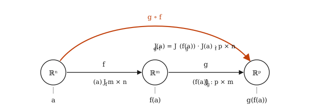
Let \(D \subseteq \mathbb{R}^n\), with \(D\) a neighbourhood of \(a\). Suppose that \(f:D \to \mathbb{R}^{m}\) is differentiable at \(a\). Let \(E \subseteq \mathbb{R}^{m}\) be a neighbourhood of \(f(a)\) with \(f(D) \subseteq E\), and \(g:E \to \mathbb{R}^{p}\) differentiable at \(f(a)\). Then \(g \circ f:D \subseteq \mathbb{R}^n\to \mathbb{R}^{p}\) is differentiable at \(a\) and moreover \(D_{g \circ f}(a) = D_{g}(f(a)) \circ D_{f}(a)\), that is, \(J_{g \circ f}(a) = J_{g}(f(a)) \cdot J_{f}(a)\) (product of a \(p \times m\) matrix by an \(m \times n\) one).

Proof: We know the following:

1. By differentiability of \(g\) at \(f(a)\), given \(\varepsilon>0\), there exists \(\delta_{1} > 0\) such that if \(\lVert h_{1} \rVert<\delta_{1}\), then

\[\lVert g(f(a)+h_{1}) - g(f(a)) - S(h_{1}) \rVert \leq \varepsilon \lVert h_{1} \rVert \quad \text{with }S = D_{g}(f(a))\]

(with \(\leq\) so that the inequality also holds when \(h_{1} = 0\)).

1. By continuity of \(f\) at \(a\), there exists \(\delta>0\) such that if \(\lVert h \rVert<\delta\), then \(\lVert f(a+h) - f(a) \rVert < \delta_{1}\).
2. By differentiability of \(f\), there exists \(\delta_{2}>0\) such that if \(\lVert h \rVert < \delta_2\) then \(\lVert f(a+h)-f(a)-T(h) \rVert < \varepsilon \lVert h \rVert\) with \(T=D_{f}(a)\).
3. By linearity of \(T\), there exists \(M>0\) such that \(\lVert T(x) \rVert \leq M \lVert x \rVert\) for every \(x\).

We must prove that \(D_{g \circ f}(a) = S \circ T\). Note that

\[\begin{aligned} \lim_{ h \to 0 } &\frac{\lVert (g \circ f)(a+h) - (g \circ f)(a) - S T (h) \rVert }{\lVert h \rVert } \\ \leq &\lim_{ h \to 0 } \underbrace{ \frac{\lVert g(f(a+h)) - g(f(a)) - S(f(a+h)-f(a))\rVert }{\lVert h \rVert } }_{ A } \\ + &\lim_{ h \to 0 }\underbrace{ \frac{\lVert S(f(a+h)-f(a)) - S(T(h))\rVert }{\lVert h \rVert } }_{ B }. \end{aligned}\]

Note that \(B = \left\lVert S\left( \frac{f(a+h)-f(a) - T(h)}{\lVert h \rVert} \right) \right\rVert\underset{h \rightarrow 0}{\longrightarrow} 0\), since \(S\) is continuous and the argument tends to zero by differentiability of \(f\). For \(A\), take \(h_{1} = f(a+h)-f(a)\) in condition (1), which is valid by (2). Then, for \(0<\lVert h \rVert < \tilde{\delta} := \min \{ \delta, \delta_{2} \}\), we have that

\[\begin{aligned} \frac{\lVert (g(f(a+h))-g(f(a)) - S(f(a+h)-f(a)) \rVert}{\lVert h \rVert } &\leq \frac{\varepsilon \lVert f(a+h) - f(a) \rVert}{\lVert h \rVert } \\ &\leq \frac{\varepsilon \lVert f(a+h) - f(a) - T(h) \rVert + \varepsilon \lVert T(h) \rVert}{\lVert h \rVert } \\ & \leq \frac{\varepsilon^{2} \lVert h \rVert + M \varepsilon \lVert h \rVert}{\lVert h \rVert } = \varepsilon^{2} + M \varepsilon, \end{aligned}\]

and since \(\varepsilon\) is arbitrary, \(A \underset{h \rightarrow 0}{\longrightarrow} 0\), from which the result follows.

Theorem (Chain rule and partial derivatives)

Let \(g=(g_{1},\dots,g_{m}):\mathbb{R}^n\to \mathbb{R}^{m}\) be of class \(C^{1}\) at \(a\) and \(f:\mathbb{R}^{m}\to \mathbb{R}^{p}\) of class \(C^{1}\) at \(g(a)\). Then \(h = f \circ g:\mathbb{R}^n\to \mathbb{R}^{p}\) is \(C^{1}\) at \(a\). Moreover, for \(i \in \{ 1,\dots,n \}\), \(j \in \{ 1,\dots,p \}\)

\[\frac{ \partial h_{j} }{ \partial x_{i} }(a) = \sum_{k=1}^{m} \frac{ \partial f_{j} }{ \partial y_{k} } (g(a)) \cdot \frac{ \partial g_{k} }{ \partial x_{i} } (a),\]

where \(y_{1},\dots,y_{m}\) denote the variables of \(f\). (The sum runs over the intermediate dimension \(m\): each variable \(y_{k}\) of \(f\) is a route through which \(x_{i}\) influences \(h_{j}\).)

Proof: We know that \(g\) is differentiable at \(a\) and \(f\) is differentiable at \(g(a)\). So, by the previous theorem, \(h\) is differentiable at \(a\) and \(J_{h}(a) =J_{f}(g(a)) J_{g}(a)\). Hence

\[\begin{aligned} \frac{ \partial h_{j} }{ \partial x_{i} }(a) = (J_{h}(a))_{ji} &= (J_{f}(g(a))J_{g}(a))_{ji}\\ &= \sum_{k=1}^{m} (J_{f}(g(a)))_{jk}(J_{g}(a))_{ki} \\ &= \sum_{k=1}^{m} \frac{ \partial f_{j} }{ \partial y_{k} } (g(a)) \cdot \frac{ \partial g_{k} }{ \partial x_{i} } (a). \end{aligned}\]

Example

Let \(f:\mathbb{R}^{2} \to \mathbb{R}\) be of class \(C^{2}\) and \(g:\mathbb{R}^{2}\to \mathbb{R}^{2}\) given by \(g(r, \theta) = (r\cos \theta, r \sin \theta)\) (polar coordinates). In this case, \(h = f \circ g:\mathbb{R}^{2}\to \mathbb{R}\) is \(h(r, \theta) = f(g_{1}, g_{2})\), with \(g_{1} = r \cos \theta\) and \(g_{2} = r \sin \theta\).

In matrix form

\[\begin{aligned} \begin{bmatrix} \frac{ \partial h }{ \partial r } & \frac{ \partial h }{ \partial \theta } \\ \end{bmatrix} \biggr\rvert_{(r, \theta)} &= \begin{bmatrix} \frac{ \partial f }{ \partial x } & \frac{ \partial f }{ \partial y } \\ \end{bmatrix} \biggr\rvert_{(g_{1},g_{2})} \begin{bmatrix} \cos \theta & -r \sin \theta \\ \sin \theta & r \cos \theta \\ \end{bmatrix} \\ &= \begin{bmatrix} \cos \theta \frac{ \partial f }{ \partial x } + \sin \theta \frac{ \partial f }{ \partial y } & -r \sin \theta \frac{ \partial f }{ \partial x } + r \cos \theta \frac{ \partial f }{ \partial y }. \end{bmatrix} \end{aligned}\]

Another way to write it is

\[D_{1} h(r, \theta) = \cos \theta \cdot D_{1} f(r \cos \theta, r \sin \theta) + \sin \theta \cdot D_{2}f(r \cos \theta, r \sin \theta).\]

The tree diagram for \(f\) and \(f_{x}\) is the following: 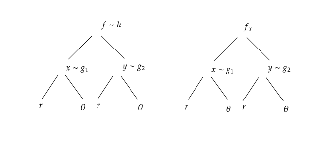The second derivative with respect to \(r\) is given by

\[\begin{aligned} \frac{ \partial^{2} h }{ \partial r^{2} } &= \frac{ \partial }{ \partial r }\left( \frac{ \partial f }{ \partial x } \frac{ \partial g_{1} }{ \partial r } + \frac{ \partial f }{ \partial y } \frac{ \partial g_{2} }{ \partial r } \right) \\ &= \frac{ \partial }{ \partial r }\left( \frac{ \partial f }{ \partial x } \right) \frac{ \partial g_{1} }{ \partial r } + \frac{ \partial f }{ \partial x } \frac{ \partial^{2} g_{1} }{ \partial r^{2} } + \frac{ \partial }{ \partial r }\left( \frac{ \partial f }{ \partial y } \right) \frac{ \partial g_{2} }{ \partial r } + \frac{ \partial f }{ \partial y } \frac{ \partial^{2} g_{2} }{ \partial r^{2} } \\ &= \left( f_{xx} \frac{ \partial g_{1} }{ \partial r } + f_{xy} \frac{ \partial g_{2} }{ \partial r } \right) \frac{ \partial g_{1} }{ \partial r } + \frac{ \partial f }{ \partial x } \underbrace{ \frac{ \partial^{2} g_{1} }{ \partial r^{2} } }_{ 0 } \\ & \quad + \left( f_{yx} \frac{ \partial g_{1} }{ \partial r } + f_{yy} \frac{ \partial g_{2} }{ \partial r } \right) \frac{ \partial g_{2} }{ \partial r } + \frac{ \partial f }{ \partial y } \underbrace{ \frac{ \partial^{2} g_{2} }{ \partial r^{2} } }_{ 0 } \\ &=f_{xx} \cos^{2} \theta + 2f_{xy} \sin \theta \cos \theta + f_{yy} \sin^{2} \theta \quad (\text{using } f_{xy} = f_{yx} \text{ by Schwarz}) \\ &=D_{11}f(r \cos \theta, r\sin \theta) \cos ^{2} \theta+ 2 D_{12} f(r \cos \theta, r \sin \theta) \sin \theta \cos \theta \\ & \quad+ D_{22} f(r \cos \theta, r \sin \theta) \sin ^{2} \theta \end{aligned}\]

Example

Let \(f:\mathbb{R}^{3}\to \mathbb{R}\), \(g,h: \mathbb{R}^{2}\to \mathbb{R}\), \(w:\mathbb{R}^{3}\to \mathbb{R}\) with

\[w(x,y,z) = f(g(x,z),h(g(x,z),y),z) = f(u,v,z)\]

with \(u=g(x,z)\), \(v=h(r,y)\) and \(r = g(x,z)\). The tree diagram records every route through which each independent variable reaches \(w\): 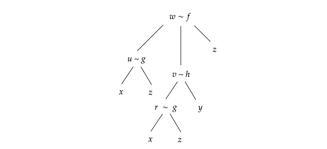Computing the first-order partial derivatives (one route per summand; note that \(z\) reaches \(w\) by three routes, one of them direct as the third variable of \(f\)):

\[\begin{aligned} \frac{ \partial w }{ \partial y } &= \frac{ \partial f }{ \partial v} \cdot \frac{ \partial h }{ \partial y } \\ \frac{ \partial w }{ \partial x } &= \frac{ \partial f }{ \partial u } \cdot \frac{ \partial g }{ \partial x } + \frac{ \partial f }{ \partial v } \cdot \frac{ \partial h }{ \partial r } \cdot \frac{ \partial g }{ \partial x } \\ \frac{ \partial w }{ \partial z } &= \frac{ \partial f }{ \partial u } \cdot \frac{ \partial g }{ \partial z } + \frac{ \partial f }{ \partial v } \cdot \frac{ \partial h }{ \partial r } \cdot \frac{ \partial g }{ \partial z } + \frac{ \partial f }{ \partial z }. \end{aligned}\]

Example (derivative along a curve)

The case \(n = 1\) is especially useful: if \(\gamma:\mathbb{R} \to \mathbb{R}^{m}\) is differentiable and \(f:\mathbb{R}^{m}\to \mathbb{R}\) is differentiable, then \(J_{\gamma}(t) = \gamma'(t)\) (a column) and \(J_{f} = \nabla f^{T}\) (a row), so

\[\frac{d}{dt} f(\gamma(t)) = J_{f}(\gamma(t)) \, J_{\gamma}(t) = \nabla f(\gamma(t)) \cdot \gamma'(t).\]

For instance, if the temperature in the plane is \(f(x,y) = x^{2}y\) and a particle follows the path \(\gamma(t) = (\cos t, \sin t)\), the temperature it feels changes at the rate

\[\frac{d}{dt}f(\gamma(t)) = (2\cos t \sin t, \cos^{2} t) \cdot (-\sin t, \cos t) = -2\cos t\sin^{2} t + \cos^{3} t,\]

which at \(t = 0\) gives \(1\); and indeed \(f(\gamma(t)) = \cos^{2}t \sin t\), whose derivative at \(0\) is \(1\). A general consequence: if \(\gamma\) moves within a level curve of \(f\) (that is, \(f \circ \gamma\) is constant), then \(\nabla f(\gamma(t)) \cdot \gamma'(t) = 0\): the gradient is normal to the level curves.

Example (the chain rule needs differentiability, not just partials)

Let \(f(x,y) = \frac{x^{2}y}{x^{2}+y^{2}}\) (with \(f(0,0) = 0\)), which we saw has \(D_{1}f(0,0) = D_{2}f(0,0) = 0\) but is not differentiable at the origin, and let \(\gamma(t) = (t,t)\). Then \(f(\gamma(t)) = \frac{t^{3}}{2t^{2}} = \frac{t}{2}\), so \(\frac{d}{dt}f(\gamma(t))\big\rvert_{t=0} = \frac{1}{2}\). But the “formula” \(\nabla f(0,0) \cdot \gamma'(0) = (0,0)\cdot(1,1) = 0\) gives something else. There is no contradiction: the chain rule requires \(f\) to be differentiable at \(\gamma(0)\), and here it is not. Having partials is not enough.

Taylor expansions

A generalisation of Taylor in one variable (MA0350). Let \(f \in C^{n+1}(V)\), \(V\) a neighbourhood of \(a\). Then the Taylor expansion of \(f\) is given by:

\[f(x) = f(a) + f'(a)(x-a) + \dots + \frac{f^{(n)}(a)}{n!}(x-a)^{n} + \frac{f^{(n+1)}(\xi)}{(n+1)!}(x-a)^{n+1}\]

with \(\xi\) between \(x\) and \(a\). Can this be generalised to functions of several variables?

Theorem (Taylor)

Let \(f:D \to \mathbb{R}\), \(f \in C^{d+1}(D)\), \(D \subseteq \mathbb{R}^n\) open. For \(a \in D\), there exists \(\delta>0\) such that for every \(x \in B_{\delta}(a)\) we have that

\[\begin{aligned} f(x) &= f(a) + \sum_{j=1}^{n} D_{j} f(a) \cdot (x_{j}-a_{j}) + \frac{1}{2!} \sum_{j_{1}=1}^{n} \sum_{j_{2}=1}^{n} D_{j_{1},j_{2}} f(a) (x_{j_{1}} - a_{j_{1}})(x_{j_{2}} - a_{j_{2}}) \\ &+ \frac{1}{3!} \sum_{j_{1},j_{2},j_{3}=1}^{n} D_{j_{1},j_{2}, j_{3}} f(a) (x_{j_{1}} - a_{j_{1}})(x_{j_{2}} - a_{j_{2}})(x_{j_{3}} - a_{j_{3}}) + \dots \\ &+ \frac{1}{d!} \sum_{j_{1},\dots,j_{d} = 1}^{n} D_{{j_{1},\dots,j_{d}}}f(a)(x_{j_{1}}-a_{j_{1}})\dots(x_{j_{d}}-a_{j_{d}}) + \\ &+ \frac{1}{(d+1)!} \sum_{j_{1},\dots,j_{d+1} = 1}^{n} D_{{j_{1},\dots,j_{d},j_{d+1}}}f(\xi)(x_{j_{1}}-a_{j_{1}})\dots(x_{j_{d}}-a_{j_{d}})(x_{j_{d+1}}-a_{j_{d+1}}), \end{aligned}\]

with \(\xi\) on the segment joining \(a\) and \(x\).

Note

Define the Hessian of \(f\) at \(a\) as the matrix of second derivatives, i.e.,

\[H_{f}(a) = \begin{pmatrix} D_{11}f(a) & D_{12}f(a) & \dots & D_{1n}f(a) \\ D_{21}f(a) & D_{22}f(a) & \dots & D_{2n}f(a) \\ \vdots & \vdots & \ddots & \vdots \\ D_{n1}f(a) & D_{n2}f(a) & \dots & D_{nn}f(a) \end{pmatrix}_{n \times n}.\]

This matrix is symmetric if \(f \in C^{2}(D)\) (Schwarz’s theorem). The second-order term of Taylor’s theorem can conveniently be written as

\[\frac{1}{2}(x-a)^{T} H_{f}(a) (x-a),\]

and the first-order one as \(\nabla f(a)^{T}(x-a) = \nabla f(a) \cdot (x-a)\).

Proof: Let \(a \in D\). Take \(B_{\delta}(a) \subseteq D\). For \(x \in B_{\delta}(a)\), define \(g:[0,1] \to \mathbb{R}\) with \(g(t) = f(\underbrace{ a+t(x-a) }_{ \in \mathbb{R}^n }) \in \mathbb{R}\). Intuitively, this function runs along the segment between \(a\) and \(x\), which is contained in the ball (the ball is convex).

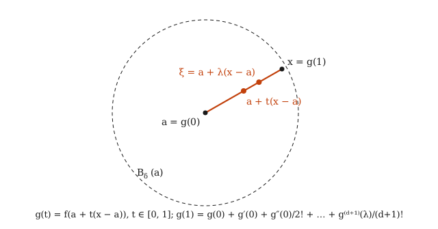
By the chain rule, \(g \in C^{d+1}[0,1]\), so Taylor’s theorem in one variable applies with \(t=1\) around \(t=0\): there exists \(\lambda \in (0,1)\) such that

\[g(1) = g(0) + g'(0) + \frac{g''(0)}{2!}+\dots + \frac{g^{(d)}(0)}{d!} + \frac{g^{(d+1)}(\lambda)}{(d+1)!}.\]

Note now that \(g(1) = f(x)\) and \(g(0) = f(a)\). Let \(v(t) = a+t(x-a)\), with components \(v_{i}(t) = a_{i}+t(x_{i} - a_{i})\) and \(v_{i}'(t) = x_{i}-a_{i}\). Expanding the derivatives with the chain rule

\[\begin{aligned} g(t) &= f(v(t)) = f\big(a_{1}+t(x_{1}-a_{1}), \dots, a_{n}+t(x_{n}-a_{n})\big)\\ \implies g'(t) &= \sum_{j=1}^{n} D_{j}f(v(t)) \cdot v_{j}'(t) = \sum_{j=1}^{n} D_{j}f(a+t(x-a)) (x_{j}-a_{j}), \\ \implies g''(t) &= \sum_{j_{1}=1}^{n} \sum_{j_{2}=1}^{n} D_{j_{1}j_{2}}f(a+t(x-a)) (x_{j_{1}}-a_{j_{1}})(x_{j_{2}}-a_{j_{2}}), \end{aligned}\]

where the second line comes from differentiating each \(D_{j_{2}}f(v(t))\) once more with the chain rule. Inductively, \(g^{(k)}(t) = \sum_{j_{1},\dots,j_{k}=1}^{n} D_{j_{1}\dots j_{k}}f(a+t(x-a))\prod_{i=1}^{k}(x_{j_{i}}-a_{j_{i}})\). Evaluating at \(t=0\) gives the terms of the expansion, and for the remainder \(\xi = a + \lambda(x-a)\), which lies on the segment between \(a\) and \(x\).

Example

Let us compute the third-order Taylor expansion of \(f(x,y) = e^{x}\sin y\) around \(a = (0,0)\). The derivatives needed are

\[\begin{aligned} f &= e^{x}\sin y, & f_{x} &= e^{x}\sin y, & f_{y} &= e^{x}\cos y, \\ f_{xx} &= e^{x}\sin y, & f_{xy} &= e^{x}\cos y, & f_{yy} &= -e^{x}\sin y, \\ f_{xxx} &= e^{x}\sin y, & f_{xxy} &= e^{x}\cos y, & f_{xyy} &= -e^{x}\sin y, & f_{yyy} &= -e^{x}\cos y, \end{aligned}\]

which at \((0,0)\) take the values \(f = 0\), \(f_{x} = 0\), \(f_{y} = 1\), \(f_{xx} = 0\), \(f_{xy} = 1\), \(f_{yy} = 0\), \(f_{xxx} = 0\), \(f_{xxy} = 1\), \(f_{xyy} = 0\), \(f_{yyy} = -1\). In the order-\(k\) sum of the theorem each mixed derivative appears as many times as its multi-index has orderings: \(f_{xy}\) appears \(2\) times (\(xy\), \(yx\)) and \(f_{xxy}\) appears \(3\) times (\(xxy\), \(xyx\), \(yxx\)). Thus,

\[\begin{aligned} f(x,y) &= \underbrace{ 0 }_{ f(a) } + \underbrace{ 0\cdot x + 1 \cdot y }_{ \text{order }1 } + \frac{1}{2!}\underbrace{ (0 \cdot x^{2} + 2 \cdot 1 \cdot xy + 0 \cdot y^{2}) }_{ \text{order }2 } + \frac{1}{3!}\underbrace{ (0 \cdot x^{3} + 3\cdot 1 \cdot x^{2}y + 3 \cdot 0 \cdot xy^{2} + (-1) y^{3}) }_{ \text{order }3 } + R_{3} \\ &= y + xy + \frac{x^{2}y}{2} - \frac{y^{3}}{6} + R_{3}(x,y), \end{aligned}\]

with \(R_{3}(x,y) = \frac{1}{4!}\sum_{j_{1},\dots,j_{4}=1}^{2} D_{j_{1}j_{2}j_{3}j_{4}}f(\xi)\, x_{j_{1}}x_{j_{2}}x_{j_{3}}x_{j_{4}}\) for some \(\xi\) on the segment from \((0,0)\) to \((x,y)\). Since all fourth-order derivatives are of the form \(\pm e^{\xi_{1}}\sin\xi_{2}\) or \(\pm e^{\xi_{1}}\cos\xi_{2}\) and \(\lvert \xi_{1} \rvert \leq \lvert x \rvert\), we get \(\lvert R_{3}(x,y) \rvert \leq \frac{e^{\lvert x \rvert}}{24}(\lvert x \rvert + \lvert y \rvert)^{4}\). Check: multiplying the series \(e^{x} = 1 + x + \frac{x^{2}}{2} + \dots\) and \(\sin y = y - \frac{y^{3}}{6} + \dots\) gives \(y + xy + \frac{x^{2}y}{2} - \frac{y^{3}}{6} + \dots\), which agrees.

Maxima and minima

Recall:

1. If \(c \in D^{0}\) is a relative extremum, \(\nabla f(c) = 0\).
2. \(f:K \subseteq \mathbb{R}^n \to \mathbb{R}\), \(K\) compact. \(f\) has absolute maximum and minimum.

Definition (Critical point)

Given \(f:D \subseteq \mathbb{R}^n \to \mathbb{R}\), we say that \(c\) is a critical point if \(f\) is not differentiable at \(c\) or if \(\nabla f(c) = 0\).

Note

Recall that being a critical point does not imply being a relative extremum. For example, \(f:\mathbb{R} \to \mathbb{R}\) with \(f(x)=x^{3}\) has a critical point at \(0\) but it is not a relative extremum. Also, \(f:\mathbb{R}^{2} \to \mathbb{R}\) with \(f(x,y) = x^{2}-y^{2}\). One can check that \(\nabla f(0,0) = 0\) but \((0,0)\) is a saddle point. We have \(f(x,0) =x^{2}\geq 0 = f(0,0)\) and \(f(0,y) = -y^{2} \leq 0 = f(0,0)\).

Definition (Maxima, minima and saddle points)

Given \(f:A \subseteq \mathbb{R}^n \to \mathbb{R}\), with \(A\) open and \(x_{0} \in A\):

1. \(f(x_{0})\) is a local maximum (resp. minimum) on \(A\) if there exists \(\rho>0\) such that \(f(x) \leq f(x_{0})\) (resp. \(f(x_{0}) \leq f(x)\)) for every \(x \in B_{\rho}(x_{0})\).
2. The extremum is global (or absolute) if the inequality holds for every \(x \in A\).
3. \(x_{0}\) is a saddle point if \(\nabla f(x_{0}) = 0\) and for every \(r>0\) with \(B_{r}(x_{0}) \subseteq A\) there exist \(x_{1}, x_{2} \in B_{r}(x_{0})\) such that \(f(x_{1}) < f(x_{0}) < f(x_{2})\).

Definition (Positive/negative definite and semidefinite matrices)

Let \(A \in \mathbb{R}^{n \times n}\) be a symmetric matrix. We say that \(A\) is:

1. positive definite if for every \(0 \neq x \in \mathbb{R}^n\), \(x^{T}Ax > 0\);
2. positive semidefinite if for every \(0 \neq x \in \mathbb{R}^n\), \(x^{T}Ax \geq 0\);
3. negative definite if for every \(0 \neq x \in \mathbb{R}^n\), \(x^{T}Ax < 0\);
4. negative semidefinite if for every \(0 \neq x \in \mathbb{R}^n\), \(x^{T}Ax \leq 0\);
5. indefinite if there exist \(0 \neq x_{1},x_{2} \in \mathbb{R}^n\) such that \(x_{1}^{T}Ax_{1}>0\) and \(x_{2}^{T} A x_{2} < 0\).

Theorem (Hessian test)

Given \(f:D \subseteq \mathbb{R}^n\to \mathbb{R}\), \(f \in C^{2}(D)\), define the Hessian matrix as

\[H_{f} = \begin{bmatrix} D_{11}f & \dots & D_{1n}f \\ \vdots & \ddots & \vdots \\ D_{n1}f & \dots & D_{nn}f \end{bmatrix}.\]

If \(\nabla f(c) = 0\) (\(c\) is a critical point), then

1. there is a relative minimum at \(c\) if \(H_{f}(c)\) is positive definite;
2. there is a relative maximum at \(c\) if \(H_{f}(c)\) is negative definite;
3. there is a relative saddle point at \(c\) if \(H_{f}(c)\) is indefinite;
4. otherwise, the test is inconclusive.

Proof: We prove case 1; case 2 follows by applying it to \(-f\). Let \(B_{\delta}(c) \subseteq D\). By Taylor’s theorem with \(d=1\) and \(\nabla f(c) = 0\), for each \(x \in B_{\delta}(c)\) there exists \(\xi\) on the segment between \(c\) and \(x\) such that

\[\begin{aligned} f(x) &= f(c) + \nabla f(c) \cdot (x-c) + \frac{1}{2} (x-c)^{T} H_{f}(\xi) (x-c)\\ \implies f(x) - f(c) &= \frac{1}{2} (x-c)^{T} H_{f}(\xi) (x-c). \end{aligned}\]

The problem is that \(H_{f}\) is evaluated at \(\xi\), not at \(c\); the continuity of the second derivatives is what lets us pass from one to the other. Since \(H_{f}(c)\) is positive definite and the unit sphere \(S = \{ u \in \mathbb{R}^n : \lVert u \rVert = 1 \}\) is compact, the continuous function \(u \mapsto u^{T}H_{f}(c)u\) attains on \(S\) a minimum \(m > 0\). By continuity of the \(D_{ij}f\) at \(c\), there exists \(0<\alpha\leq\delta\) such that \(\lvert D_{ij}f(\xi) - D_{ij}f(c) \rvert < \frac{m}{2n^{2}}\) for all \(i,j\) whenever \(\lVert \xi - c \rVert < \alpha\). Then, for \(u \in S\) and such \(\xi\),

\[\lvert u^{T} H_{f}(\xi) u - u^{T} H_{f}(c) u \rvert \leq \sum_{i,j=1}^{n} \lvert D_{ij}f(\xi) - D_{ij}f(c) \rvert \, \lvert u_{i} \rvert \lvert u_{j} \rvert < n^{2} \cdot \frac{m}{2n^{2}} = \frac{m}{2},\]

so that \(u^{T}H_{f}(\xi)u > m - \frac{m}{2} = \frac{m}{2} > 0\). If \(0<\lVert x-c \rVert < \alpha\), then \(\xi \in B_{\alpha}(c)\) and, writing \(x - c = \lVert x-c \rVert u\) with \(u \in S\),

\[f(x) - f(c) = \frac{\lVert x-c \rVert^{2}}{2} \, u^{T} H_{f}(\xi) u > \frac{m}{4}\lVert x-c \rVert^{2} > 0.\]

We conclude that \(f(c)\) is a (strict) relative minimum. For case 3, if \(H_{f}(c)\) is indefinite, take \(u_{1},u_{2} \in S\) with \(u_{1}^{T}H_{f}(c)u_{1} > 0 > u_{2}^{T}H_{f}(c)u_{2}\); the same continuity argument, applied along each direction, shows that \(f(c+tu_{1}) > f(c)\) and \(f(c+tu_{2}) < f(c)\) for small \(t>0\), so \(c\) is a saddle point.

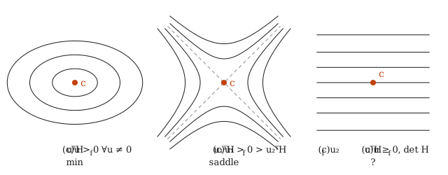
Theorem (Characterisation of definite and semidefinite matrices)

Let \(A\) be symmetric. The following are equivalent:

1. \(A\) is positive (resp. negative) definite;
2. the eigenvalues of \(A\) are all positive (resp. negative);
3. the determinants of the leading principal minors \(\Delta_{k} = \det(A_{1..k,1..k})\), \(k=1,\dots,n\), are all positive (resp. alternate in sign starting with a negative one: \((-1)^{k}\Delta_{k} > 0\)).

Moreover, the following are equivalent:

1. \(A\) is indefinite;
2. \(A\) has both negative and positive eigenvalues.

For \(n=2\) the test is especially convenient: with \(\Delta_{2} = \det A\), if \(\Delta_{2}<0\) the matrix is indefinite (the eigenvalues have opposite signs, since their product is \(\det A\)); if \(\Delta_{2}>0\) it is definite, with the sign of \(\Delta_{1} = a_{11}\); and if \(\Delta_{2} = 0\) it is semidefinite and the Hessian test is inconclusive. Warning: criterion (3) does not extend to semidefinite matrices by replacing \(>\) with \(\geq\) (for instance \(\begin{bmatrix} 0 & 0 \\ 0 & -1 \end{bmatrix}\) has \(\Delta_{1} = \Delta_{2} = 0\) and is not positive semidefinite); for those one has to check all the principal minors, or use the eigenvalues.

Example

Consider \(f(x,y) = x^{3}-3xy^{2}+y^{2}\). First, we find the critical points.

Note that \(\nabla f(x,y) = (3x^{2}-3y^{2}, -6xy+2y) = (0,0)\)

\[\implies \begin{cases} x ^{2} = y^{2} \\ -3xy+y=0 \end{cases}.\]

We have \((0,0), \left( \frac{1}{3}, \frac{1}{3} \right), \left( \frac{1}{3}, -\frac{1}{3} \right)\) as critical points. The Hessian of \(f\) is

\[H_{f}(x,y) = \begin{bmatrix} 6x & -6y \\ -6y & -6x+2 \end{bmatrix}.\]

Finally, we compute the determinants of the minors in each case:

\[\begin{aligned} H_{f}\left( \frac{1}{3}, \frac{1}{3} \right) &= \begin{bmatrix} 2 & -2 \\ -2 & 0 \end{bmatrix} \implies \Delta_{1} = 2 > 0, \ \Delta_{2} = -4 < 0 \quad \text{(indefinite)}, \\ H_{f}\left( \frac{1}{3}, \frac{-1}{3} \right) &= \begin{bmatrix} 2 & 2 \\ 2 & 0 \end{bmatrix} \implies \Delta_{1} = 2 > 0, \ \Delta_{2} = -4 <0 \quad \text{(indefinite)}. \end{aligned}\]

So both points are saddle points. For the point \((0,0)\) we have \(H_{f}(0,0) = \begin{bmatrix} 0 & 0 \\ 0 & 2 \end{bmatrix}\), so \(\Delta_{1} = \Delta_{2} = 0\) and \((x,y)H_{f}(0,0) (x,y)^{T} = 2y^{2} \geq 0\): the matrix is positive semidefinite but not positive definite, and the test is inconclusive. It is tempting to conclude that there is a minimum, but that is false: on the \(x\)-axis, \(f(x,0) = x^{3}\), which is positive for \(x>0\) and negative for \(x<0\), whereas \(f(0,0) = 0\). Every ball around \((0,0)\) contains points with \(f>0\) and points with \(f<0\), so \((0,0)\) is a saddle point, not an extremum. Moral: semidefinite is not enough; when the test is inconclusive, one has to look at the function directly.

Example (when the test is inconclusive, anything can happen)

The functions \(f_{1}(x,y) = x^{4}+y^{4}\), \(f_{2}(x,y) = x^{4}-y^{4}\) and \(f_{3}(x,y) = x^{3}+y^{2}\) all have \((0,0)\) as a critical point; the Hessian there is the zero matrix for the first two and \(\begin{bmatrix} 0 & 0 \\ 0 & 2 \end{bmatrix}\) (positive semidefinite) for the third, so the test is inconclusive in all three cases. Nevertheless, \((0,0)\) is a strict minimum of \(f_{1}\), a saddle point of \(f_{2}\) (since \(f_{2}(x,0) = x^{4} > 0 > -y^{4} = f_{2}(0,y)\)) and a saddle point of \(f_{3}\) (since \(f_{3}(x,0) = x^{3}\) changes sign). In these cases one has to analyse \(f\) directly, typically by restricting it to lines or curves through the critical point.

Example (three variables)

Let \(f(x,y,z) = x^{2}+y^{2}+z^{2}-xy-yz\). Then \(\nabla f = (2x - y,\ 2y - x - z,\ 2z - y)\), which vanishes only at the origin (the system is linear and its matrix has determinant \(4 \neq 0\)), and

\[H_{f} = \begin{bmatrix} 2 & -1 & 0 \\ -1 & 2 & -1 \\ 0 & -1 & 2 \end{bmatrix}, \qquad \Delta_{1} = 2, \quad \Delta_{2} = \det\begin{bmatrix} 2 & -1 \\ -1 & 2 \end{bmatrix} = 3, \quad \Delta_{3} = \det H_{f} = 4.\]

All positive, so \(H_{f}\) is positive definite and \((0,0,0)\) is a relative minimum; in fact it is absolute, since \(f(x) = \frac{1}{2}x^{T}H_{f}x > 0 = f(0)\) for every \(x \neq 0\).

Example (absolute extrema on a compact set)

Let \(f(x,y) = x^{2}+2y^{2}-x\) on the closed disc \(K = \{ (x,y) : x^{2}+y^{2} \leq 1 \}\). Since \(K\) is compact and \(f\) is continuous, an absolute maximum and an absolute minimum exist, and each is attained either at a critical point of the interior or on the boundary.

Interior: \(\nabla f = (2x-1, 4y) = (0,0) \iff (x,y) = \left( \frac{1}{2},0 \right)\), which lies in the interior of \(K\), with \(f\left( \frac{1}{2},0 \right) = -\frac{1}{4}\).

Boundary: we parametrise \(x^{2}+y^{2} = 1\) by \((\cos t, \sin t)\) and study \(\varphi(t) = f(\cos t,\sin t) = \cos^{2}t + 2\sin^{2}t - \cos t = 2 - \cos^{2}t - \cos t\). With \(c = \cos t \in [-1,1]\), the function \(2 - c^{2} - c\) has derivative \(-2c-1\), which vanishes at \(c = -\frac{1}{2}\), where it equals \(\frac{9}{4}\); at the endpoints, \(c = 1\) gives \(0\) and \(c = -1\) gives \(2\).

Comparing: the absolute minimum is \(-\frac{1}{4}\), at \(\left( \frac{1}{2},0 \right)\), and the absolute maximum is \(\frac{9}{4}\), attained at the two boundary points with \(\cos t = -\frac{1}{2}\): \(\left( -\frac{1}{2}, \pm\frac{\sqrt{ 3 }}{2} \right)\). Note that on the boundary \(\nabla f\) is not used (those points are not critical points of \(f\)): the boundary problem is a one-variable problem.

Differentiation of inverses and the implicit function theorem

Example

If \(f:\mathbb{R}\to \mathbb{R}\) is invertible and differentiable, with differentiable inverse \(g=f^{-1}\), we know that \(g(f(x))= x\). By the chain rule, \(g'(f(x)) f'(x) = 1\) and so \(g'(y)=\frac{1}{f'(f^{-1}(y))}\), where \(y = f(x)\) and \(f'(x) \neq 0\). Note that the argument assumes that \(g\) is differentiable; the inverse function theorem is precisely what guarantees this (and the local existence of \(g\)) from \(f'(x) \neq 0\).

Example

To compute \(g'\) for \(g(x)=\arcsin x \in \left[ -\frac{\pi}{2}, \frac{\pi}{2} \right]\). We know that \(\sin(g(x)) = x\) and so \(\cos(g(x)) g'(x) = 1\). Thus

\[g'(x) = \frac{1}{\cos(g(x))} = \frac{1}{\sqrt{ 1 - \sin^{2}(g(x)) }} = \frac{1}{\sqrt{ 1-x^{2} }}.\]

It is enough to know that \((\sin x)' = \cos x \neq 0\) for every \(x \in (-\frac{\pi}{2}, \frac{\pi}{2})\) to know that \(\sin\) is locally invertible there, with differentiable inverse (for \(x = \pm 1\), the endpoints of the domain of \(\arcsin\), the derivative blows up: \(\cos(\pm\frac{\pi}{2}) = 0\)).

Theorem (Inverse function theorem)

Let \(f:A \subseteq \mathbb{R}^n \to \mathbb{R}^n\), \(f \in C^{1}(A)\) with \(A\) open. Let \(a \in A\) with \(\det J_{f}(a) \neq 0\). Then:

1. there exist open \(V,W \subseteq\mathbb{R}^n\) such that \(a \in V\), \(f(a) \in W\) and \(f:V\to W\) is bijective, with \(f^{-1}:W\to V\) of class \(C^{1}\);
2. \(J_{f^{-1}}(y)= [J_{f}(f^{-1}(y))]^{-1}\) for every \(y \in W\).

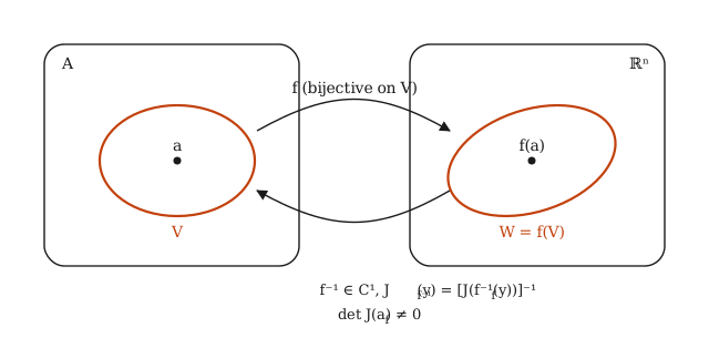
Idea of the proof: (In class this was left to a supplementary video; this is the structure of the argument.)

1. Formula for the derivative. If we already know that \(f^{-1}\) exists on \(W\) and is differentiable, the chain rule applied to \(f^{-1} \circ f = \mathrm{id}_{V}\) gives \(J_{f^{-1}}(f(x)) \cdot J_{f}(x) = I\), which is (2). The hard part is (1) and the differentiability of the inverse.
2. Reduction. Composing with the invertible linear transformation \(J_{f}(a)^{-1}\) (which affects none of the conclusions), we may assume \(J_{f}(a) = I\). By continuity of the partials, there is a closed ball \(\bar B = \bar B_{r}(a)\) on which \(\lVert J_{f}(x) - I \rVert < \frac{1}{2}\) and \(\det J_{f}(x) \neq 0\).
3. Injectivity. Let \(\varphi(x) = x - f(x)\), so that \(J_{\varphi} = I - J_{f}\) has norm less than \(\frac{1}{2}\) on \(\bar B\). By the mean value theorem applied to each component, \(\lVert \varphi(x) - \varphi(x') \rVert \leq \frac{1}{2}\lVert x-x' \rVert\) for \(x,x' \in \bar B\), and then

\[\lVert f(x) - f(x') \rVert \geq \lVert x-x' \rVert - \lVert \varphi(x)-\varphi(x') \rVert \geq \tfrac{1}{2}\lVert x-x' \rVert.\]

So \(f\) is injective on \(\bar B\) and its inverse (where it exists) is Lipschitz, in particular continuous.

1. The image is open. Let \(V = B_{r}(a)\) and \(W = f(V)\). Given \(y_{0} = f(x_{0})\) with \(x_{0} \in V\), take \(\rho>0\) with \(\bar B_{\rho}(x_{0}) \subseteq V\) and let \(y\) satisfy \(\lVert y - y_{0} \rVert < \frac{\rho}{4}\). The function \(x \mapsto \lVert f(x) - y \rVert^{2}\) is continuous on the compact set \(\bar B_{\rho}(x_{0})\) and attains its minimum. On the sphere \(\lVert x - x_{0} \rVert = \rho\), by step 3, \(\lVert f(x) - y \rVert \geq \lVert f(x) - y_{0} \rVert - \lVert y - y_{0} \rVert \geq \frac{\rho}{2} - \frac{\rho}{4} > \lVert f(x_{0}) - y \rVert\), so the minimum is not on the boundary. At an interior minimum the gradient vanishes: \(2 J_{f}(x)^{T}(f(x)-y) = 0\), and since \(J_{f}(x)\) is invertible, \(f(x) = y\). Hence \(B_{\rho/4}(y_{0}) \subseteq W\): \(W\) is open, and \(f:V \to W\) is bijective by step 3.
2. Differentiability of the inverse. Let \(y = f(x)\), \(y+k = f(x+h)\) with \(T = J_{f}(x)\). Then \(k = T h + r(h)\) with \(\lVert r(h) \rVert / \lVert h \rVert \to 0\), and

\[f^{-1}(y+k) - f^{-1}(y) - T^{-1}k = h - T^{-1}(Th + r(h)) = -T^{-1} r(h).\]

Since \(\lVert h \rVert \leq 2\lVert k \rVert\) by step 3, \(\frac{\lVert T^{-1}r(h) \rVert}{\lVert k \rVert} \leq 2\lVert T^{-1} \rVert \frac{\lVert r(h) \rVert}{\lVert h \rVert} \to 0\) as \(k \to 0\) (which forces \(h \to 0\)). Therefore \(f^{-1}\) is differentiable at \(y\) with \(D_{f^{-1}}(y) = J_{f}(x)^{-1}\), and since \(y \mapsto J_{f}(f^{-1}(y))^{-1}\) is continuous (the entries of the inverse are quotients of polynomials in the entries, with the determinant as denominator), \(f^{-1} \in C^{1}(W)\).

Note

1. The theorem is local: \(f\) may fail to be globally injective even though \(\det J_{f} \neq 0\) everywhere (see the second example).
2. The condition \(\det J_{f}(a) \neq 0\) is sufficient but not necessary for an inverse to exist: \(f(x) = x^{3}\) is a bijection of \(\mathbb{R}\) with \(f'(0) = 0\); what is lost is the differentiability of the inverse at \(0\) (\(\sqrt[3]{y}\) is not differentiable at \(0\)).
3. If \(f \in C^{k}\), then \(f^{-1} \in C^{k}\) (iterate the continuity argument of step 5).

Example (polar coordinates)

Let \(f(r,\theta) = (r\cos\theta, r\sin\theta)\), of class \(C^{\infty}\) on \(\mathbb{R}^{2}\). Then

\[J_{f}(r,\theta) = \begin{bmatrix} \cos\theta & -r\sin\theta \\ \sin\theta & r\cos\theta \end{bmatrix}, \qquad \det J_{f}(r,\theta) = r\cos^{2}\theta + r\sin^{2}\theta = r.\]

Thus, at every point with \(r \neq 0\) the theorem gives a local \(C^{1}\) inverse (a local determination of \((x,y) \mapsto (\sqrt{x^{2}+y^{2}}, \theta)\)), with

\[J_{f^{-1}}(x,y) = [J_{f}(r,\theta)]^{-1} = \frac{1}{r}\begin{bmatrix} r\cos\theta & r\sin\theta \\ -\sin\theta & \cos\theta \end{bmatrix} = \begin{bmatrix} \frac{x}{\sqrt{ x^{2}+y^{2} }} & \frac{y}{\sqrt{ x^{2}+y^{2} }} \\ -\frac{y}{x^{2}+y^{2}} & \frac{x}{x^{2}+y^{2}} \end{bmatrix},\]

which agrees with differentiating \(r = \sqrt{x^{2}+y^{2}}\) and \(\theta = \arctan(y/x)\) directly. At \(r = 0\) the theorem does not apply, and indeed \(f\) is not injective on any neighbourhood of the axis \(r=0\) (every \((0,\theta)\) is sent to the origin).

Example (local but not global)

Let \(f(x,y) = (e^{x}\cos y, e^{x}\sin y)\). Then

\[J_{f}(x,y) = \begin{bmatrix} e^{x}\cos y & -e^{x}\sin y \\ e^{x}\sin y & e^{x}\cos y \end{bmatrix}, \qquad \det J_{f}(x,y) = e^{2x} > 0\]

on all of \(\mathbb{R}^{2}\), so \(f\) is locally invertible at every point. However, \(f(x,y+2\pi) = f(x,y)\): \(f\) is not injective on \(\mathbb{R}^{2}\) and has no global inverse. (It is the complex exponential \(z \mapsto e^{z}\) seen in \(\mathbb{R}^{2}\); the local inverses are the branches of the logarithm.)

Example (computing a derivative of the inverse without knowing the inverse)

Let \(f(x,y) = (x+y, xy)\) and \(a = (2,1)\), with \(f(a) = (3,2)\). Since \(J_{f}(x,y) = \begin{bmatrix} 1 & 1 \\ y & x \end{bmatrix}\) and \(\det J_{f}(2,1) = 2-1 = 1 \neq 0\), there is a local inverse \(g = f^{-1}\) near \((3,2)\) with \(g(3,2) = (2,1)\), and

\[J_{g}(3,2) = [J_{f}(2,1)]^{-1} = \begin{bmatrix} 1 & 1 \\ 1 & 2 \end{bmatrix}^{-1} = \begin{bmatrix} 2 & -1 \\ -1 & 1 \end{bmatrix}.\]

This says, for instance, that if the sum \(s = x+y\) increases by \(\Delta s\) and the product \(p = xy\) stays fixed, then \(x\) increases by approximately \(2\Delta s\) and \(y\) decreases by approximately \(\Delta s\). Note that on the line \(x = y\) the determinant vanishes: there \(f\) is not locally injective, since \(f(x,y) = f(y,x)\) and the points \((x,y)\) and \((y,x)\) approach each other as they approach the diagonal.

Theorem (Implicit function theorem)

Let \(f:\mathbb{R}^n \times \mathbb{R}^{m} \to \mathbb{R}^{m}\) be of class \(C^{1}\) on an open set containing \((a,b)\), with \(a \in \mathbb{R}^n\), \(b \in \mathbb{R}^{m}\), \(f(a,b)=0\). Let \(M \in \mathbb{R}^{m \times m}\) with \(M_{ij} = D_{n+j}f_{i}\), \(1\leq i,j\leq m\). If \(\det M(a,b) \neq 0\), there exist \(A \subseteq \mathbb{R}^n\), \(B \subseteq \mathbb{R}^{m}\) with \(a \in A\), \(b \in B\) such that

\[\forall x \in A \quad \exists ! y \in B \quad (f(x,y)=0).\]

That is, there exists a unique \(g :A\to B\) with \(f(x, g(x)) = 0\) for every \(x \in A\) (and \(g(a) = b\)). Moreover, \(g\) is of class \(C^{1}\) on \(A\) and \(J_{g}(x) = -[M(x,g(x))]^{-1} N(x,g(x))\), where \(N = [D_{j}f_{i}]_{1\leq i\leq m, \hspace{1mm} 1\leq j\leq n}\) is the block of \(J_{f}\) corresponding to the \(x\) variables.

Idea of the proof: We can write the Jacobian of \(f\) as

\[\begin{aligned} J_{f} &= \begin{bmatrix} N & M \\ \end{bmatrix}_{m \times (n+m)}, \\ \\ \text{with }N &= \begin{bmatrix} D_{1}f_{1} & \dots & D_{n}f_{1} \\ \vdots & \ddots & \vdots \\ D_{1}f_{m} & \dots & D_{n}f_{m} \\ \end{bmatrix}_{m \times n} \text{and } M = \begin{bmatrix} D_{n+1}f_{1} & \dots & D_{n+m} f_{1} \\ \vdots & \ddots & \vdots \\ D_{n+1}f_{m} & \dots & D_{n+m}f_{m} \end{bmatrix}_{m \times m}. \end{aligned}\]

Let \(h:\mathbb{R}^n \to \mathbb{R}^{n+m}\) with \(h(x) = (x,g(x))\); we have that \(J_{h} = \begin{bmatrix}I_{n\times n} \\ J_{g}\end{bmatrix}\). Since \(f \circ h = 0\), we have that

\[0 = \begin{bmatrix} N & M \end{bmatrix} \begin{bmatrix} I \\ J_{g} \end{bmatrix} = N+MJ_{g} \implies J_{g} = -M^{-1}N.\]

Example

Consider the circle \(x^{2}+y^{2} = 1\), that is, the zero set of \(f(x,y) = x^{2}+y^{2}-1\). Here \(n = m = 1\) and \(M = \frac{ \partial f }{ \partial y } = 2y\), which is nonzero except at \((-1,0)\) and \((1,0)\). Around any other point \((a,b)\) of the circle, the theorem guarantees an interval \(A\) around \(a\) and a unique function \(y = g(x)\) with \(g(a) = b\) and \(x^{2}+g(x)^{2} = 1\); concretely \(g(x) = \sqrt{ 1-x^{2} }\) if \(b>0\) and \(g(x) = -\sqrt{ 1-x^{2} }\) if \(b<0\). At \((\pm 1, 0)\) there is no such function: every interval around \(x = 1\) contains points \(x>1\) with no preimage and points \(x<1\) with two (\(\pm\sqrt{ 1-x^{2} }\)); geometrically, the tangent is vertical. Differentiating implicitly with respect to \(x\), thinking of \(y = y(x)\): \(2x + 2y\,y' = 0\), hence \(y' = -\frac{x}{y} = -\frac{f_{x}}{f_{y}}\), which is the formula of the theorem.

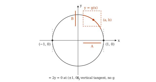
Special case

For \(n=m=1\), we have \(f:\mathbb{R} \times \mathbb{R} \to \mathbb{R}\), so \(N = \frac{ \partial f }{ \partial x }\) and \(M = \frac{ \partial f }{ \partial y }\). If \(\det\left( \frac{ \partial f }{ \partial y } \right) \neq 0\), \(\frac{dy}{dx} = -\frac{\frac{ \partial f }{ \partial x }}{\frac{ \partial f }{ \partial y }}\).

Example

Consider \(f(x,y) = \ln x+2\ln y+xy-1\) for \(x,y>0\) and \((a,b)=(1,1)\). Note that \(f(1,1) = 0 + 0 + 1 - 1 = 0\) and that \(M = \frac{ \partial f }{ \partial y } = \frac{2}{y} + x \implies M(1,1) = 3 \neq 0\). By the implicit function theorem, there exist open subsets \(A,B\) of \(\mathbb{R}\), with \(1 \in A\), \(1 \in B\), and a unique \(g:A \to B\) of class \(C^{1}\) with \(g(1) = 1\) and \(f(x,g(x)) = 0\). Although we cannot solve for \(g\) explicitly, we can differentiate it:

\[g'(1) = -\frac{f_{x}(1,1)}{f_{y}(1,1)} = -\frac{\frac{1}{x}+y}{\frac{2}{y}+x}\Bigg\rvert_{(1,1)} = -\frac{2}{3}.\]

So, near \(x = 1\), \(g(x) \approx 1 - \frac{2}{3}(x-1)\).

Example (a surface as a local graph)

Let \(F(x,y,z) = xz + yz^{2} + z^{3} - 1\) and \((a,b) = ((0,0), 1)\), with \(n = 2\), \(m = 1\). We have \(F(0,0,1) = 0\) and \(M = F_{z} = x + 2yz + 3z^{2}\), with \(M(0,0,1) = 3 \neq 0\). Hence near \((0,0)\) the surface \(F = 0\) is the graph of a function \(z = g(x,y)\) of class \(C^{1}\) with \(g(0,0) = 1\), and

\[J_{g}(0,0) = -M^{-1}N = -\frac{1}{F_{z}}\begin{bmatrix} F_{x} & F_{y} \end{bmatrix}\Bigg\rvert_{(0,0,1)} = -\frac{1}{3}\begin{bmatrix} z & z^{2} \end{bmatrix}\Bigg\rvert_{(0,0,1)} = \begin{bmatrix} -\frac{1}{3} & -\frac{1}{3} \end{bmatrix}.\]

The tangent plane to the surface at \((0,0,1)\) is therefore \(z = 1 - \frac{x}{3} - \frac{y}{3}\). Note that it is the same plane given by \(\nabla F(0,0,1) \cdot (x,y,z-1) = 0\), since \(\nabla F(0,0,1) = (1,1,3)\).

Example (two equations, \(m = 2\))

Consider the system

\[\begin{cases} F_{1}(x,y,z) = x^{2}+y^{2}+z^{2}-3 = 0 \\ F_{2}(x,y,z) = xy - z = 0 \end{cases}\]

near the point \((1,1,1)\), which satisfies it. Can we solve for \((y,z)\) as functions of \(x\)? Here \(n = 1\), \(m = 2\), and the block of the dependent variables is

\[M = \frac{ \partial (F_{1},F_{2}) }{ \partial (y,z) } = \begin{bmatrix} 2y & 2z \\ x & -1 \end{bmatrix}, \qquad M(1,1,1) = \begin{bmatrix} 2 & 2 \\ 1 & -1 \end{bmatrix}, \qquad \det M(1,1,1) = -4 \neq 0.\]

By the theorem, there exists \(g(x) = (y(x), z(x))\) of class \(C^{1}\) near \(x = 1\) with \(g(1) = (1,1)\), and with \(N = \frac{ \partial (F_{1},F_{2}) }{ \partial x } = \begin{bmatrix} 2x \\ y \end{bmatrix}\),

\[J_{g}(1) = \begin{bmatrix} y'(1) \\ z'(1) \end{bmatrix} = -M^{-1}N = -\frac{1}{-4}\begin{bmatrix} -1 & -2 \\ -1 & 2 \end{bmatrix}\begin{bmatrix} 2 \\ 1 \end{bmatrix} = \frac{1}{4}\begin{bmatrix} -4 \\ 0 \end{bmatrix} = \begin{bmatrix} -1 \\ 0 \end{bmatrix}.\]

Check by implicit differentiation: differentiating both equations with respect to \(x\) at \((1,1,1)\) gives \(2 + 2y' + 2z' = 0\) and \(1 + y' - z' = 0\), whose solution is \(y' = -1\), \(z' = 0\). Geometrically, the curve of intersection of the sphere with the saddle \(z = xy\) passes through \((1,1,1)\) with tangent vector \((1,-1,0)\).

Note

If \(\det M(a,b) = 0\) the theorem says nothing, and anything can happen: for \(f(x,y) = y^{2} - x^{2}\) at \((0,0)\) there is no unique function \(y = g(x)\) (there are two: \(\pm x\)), whereas for \(f(x,y) = y^{3} - x\) at \((0,0)\) there is a unique one, \(g(x) = \sqrt[3]{x}\), but it is not differentiable at \(0\).

Closing remarks

Directional derivative and gradient

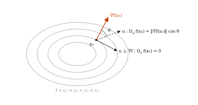
Given \(u \in \mathbb{R}^n\) with \(\lVert u \rVert_{2} = 1\) and \(f:\mathbb{R}^n\to \mathbb{R}\) differentiable at \(x_{0}\), then \(D_{u}f(x_{0}) = \nabla f(x_{0}) \cdot u\) and, by Cauchy-Schwarz,

\[\begin{aligned} \lvert D_{u} f(x_{0}) \rvert &= \lvert \nabla f(x_{0}) \cdot u \rvert \\ &= \lVert \nabla f(x_{0}) \rVert \cdot \lVert u \rVert \lvert \cos \theta \rvert = \lVert \nabla f(x_{0}) \rVert \cdot \lvert \cos \theta \rvert \\ &\leq \lVert \nabla f(x_{0}) \rVert, \end{aligned}\]

where \(\theta\) is the angle between \(\nabla f(x_{0})\) and \(u\). If \(u, \nabla f(x_{0})\) are parallel, equality holds, since \(\theta = 0 \implies \cos \theta = 1\).

If \(\nabla f(x_{0}) \neq 0\) and I take \(u = \frac{\nabla f(x_{0})}{\lVert \nabla f(x_{0}) \rVert}\), then \(D_{u} f(x_{0}) = \lVert \nabla f(x_{0}) \rVert\) is the largest possible value: \(\nabla f(x_{0})\) points in the direction of greatest increase of \(f\) at \(x_{0}\), and \(-\nabla f(x_{0})\) in that of greatest decrease. In the directions perpendicular to the gradient (\(\theta = \pi/2\)) the directional derivative is zero: these are the directions tangent to the level curve \(\{ f = f(x_{0}) \}\), so the gradient is normal to the level curves.

Example

Let \(f(x,y) = x^{2}y\) and \(x_{0} = (1,2)\). Then \(\nabla f(x,y) = (2xy, x^{2})\) and \(\nabla f(1,2) = (4,1)\). In the direction \(u = \left( \frac{3}{5}, \frac{4}{5} \right)\),

\[D_{u}f(1,2) = \nabla f(1,2) \cdot u = \frac{12}{5} + \frac{4}{5} = \frac{16}{5},\]

whereas the maximum rate of increase at \((1,2)\) is \(\lVert \nabla f(1,2) \rVert = \sqrt{ 17 }\), attained in the direction \(\frac{(4,1)}{\sqrt{ 17 }}\), and in the direction \(\frac{(1,-4)}{\sqrt{ 17 }}\), tangent to the level curve \(x^{2}y = 2\), the directional derivative is zero.

Higher-order differentials.

Given \(f:A \subseteq \mathbb{R}^n \to \mathbb{R}\) differentiable, at each point we have \(D_{f}(x_{0}):\mathbb{R}^n\to \mathbb{R}\) linear, with \(D_{f}(x_{0})(h) \in \mathbb{R}\). We may therefore view the derivative as a function \(D_{f}: A \to \mathcal{L}(\mathbb{R}^n, \mathbb{R})\) assigning a linear transformation to each point. We saw that \(D_{f}(x)\) has \(J_{f}(x)\) as its associated matrix. So

\[D_{f}(x_{0}) (h) = J_{f}(x_{0}) h = \sum_{i=1}^{n} \frac{ \partial f }{ \partial x_{i} } (x_{0}) h_{i}.\]

It makes sense to define \(D(D_{f}(x_{0}))\) if \(f \in C^{2}(A)\).

If \(x = (x_{1},\dots,x_{n})\), it is usual to define projections \(dx_{i}:\mathbb{R}^n\to \mathbb{R}\) with \(dx_{i}(x) = x_{i}\). So \(D_{f}(x_{0}) = \sum_{i=1}^{n} \frac{ \partial f(x_{0}) }{ \partial x_{i} } dx_{i}\). Evaluating, \(D_{f}(x_{0})(h) = \sum_{i=1}^{n} \frac{ \partial f(x_{0}) }{ \partial x_{i} } dx_{i}(h)\). So

\[\begin{aligned} \implies D(D_{f}(x_{0})) &= \sum_{j=1}^{n} \frac{ \partial }{ \partial x_{j} }(D_{f}(x_{0})) dx_{j} \\ &= \sum_{j=1}^{n} \frac{ \partial }{ \partial x_{j} } \left( \sum_{i=1}^{n} \frac{ \partial f(x_{0}) }{ \partial x_{i} } dx_{i}(h) \right) dx_{j} \\ &= \sum_{i,j=1}^{n} \frac{ \partial^{2} f }{ \partial x_{j} \partial x_{i} } dx_{i} dx_{j}, \quad \text{with } dx_{i} dx_{j}: \mathbb{R}^n \times \mathbb{R}^n \\ \implies D_{f}^{2}(x_{0})(u,v) &= \sum_{i,j=1}^{n} \frac{ \partial^{2} f }{ \partial x_{j} \partial x_{i} }(x_{0}) u_{i} v_{j} \quad= u^{T} H v. \end{aligned}\]

Definition (Higher-order differential)

Let \(B_{2}(\mathbb{R}^n,\mathbb{R}) = \{ f:D\to \mathbb{R} \text{ bilinear}\}\), with \(D = \{ (x,x): x \in \mathbb{R}^n \}\). Define \(D^{2}f:A \subseteq \mathbb{R}^n \to B_{2}(\mathbb{R}^n, \mathbb{R})\) by

\[(D^{2}f(x_{0}))(x) = x^{T} H_{f}(x_{0}) x = \sum_{i,j=1}^{n} x_{i} x_{j} \frac{ \partial^{2} f }{ \partial x_{i} \partial x_{j} }(x_{0}).\]

Analogously, \(D^{3}f:A \subseteq \mathbb{R}^n \to B_{3}(\mathbb{R}^{n}, \mathbb{R})\) given by

\[(D^{3}f(x_{0}))(x) = \sum_{i,j,k=1}^{n} x_{i} x_{j} x_{k} f_{x_{k}x_{j}x_{i}}(x_{0}),\]

where \(B_{3}\) is the set of trilinear functions restricted to \((x,x,x)\) with \(x \in \mathbb{R}^n\).

Note

Taylor can be rewritten as

\[f(x) = f(x_{0}) + \sum_{k=1}^{p} \frac{1}{k!} (D^{k}f(x_{0}))(x-x_{0}) + \frac{1}{(p+1)!}(D^{p+1}f(\xi))(x-x_{0}).\]

Example

Let \(f(x,y) = x^{2}y\) and \(x_{0} = (1,2)\). Then \(\nabla f(1,2) = (4,1)\) and \(H_{f}(x,y) = \begin{bmatrix} 2y & 2x \\ 2x & 0 \end{bmatrix}\), so \(H_{f}(1,2) = \begin{bmatrix} 4 & 2 \\ 2 & 0 \end{bmatrix}\). For \(h = (h_{1},h_{2})\),

\[D^{1}f(1,2)(h) = 4h_{1} + h_{2}, \qquad D^{2}f(1,2)(h) = h^{T}H_{f}(1,2)h = 4h_{1}^{2} + 4h_{1}h_{2}, \qquad D^{3}f(1,2)(h) = 3 f_{xxy}\, h_{1}^{2}h_{2} = 6h_{1}^{2}h_{2},\]

since the only nonzero third derivative is \(f_{xxy} = f_{xyx} = f_{yxx} = 2\) (three orderings of the same index) and those of order 4 and higher are zero. Since the fourth-order remainder vanishes, Taylor is exact:

\[f(1+h_{1},2+h_{2}) = 2 + (4h_{1}+h_{2}) + \frac{1}{2}(4h_{1}^{2}+4h_{1}h_{2}) + \frac{1}{6}\cdot 6h_{1}^{2}h_{2} = 2 + 4h_{1} + h_{2} + 2h_{1}^{2} + 2h_{1}h_{2} + h_{1}^{2}h_{2},\]

which is indeed the expansion of \((1+h_{1})^{2}(2+h_{2})\).