Curves
Definition (Curve of class \(C^{p}\))
- Given an interval \(I \subseteq \mathbb{R}\), a function \(\gamma:I \to \mathbb{R}^n\) is of class \(C^{p}(I)\) if there exists an open set \(J\) with \(I \subset J\) and \(\tilde{\gamma}: J\to \mathbb{R}^n\) such that \(\tilde{\gamma} \in C^{p}(J)\) (the usual definition for open intervals) with \(\tilde{\gamma}(t) = \gamma(t)\) for every \(t \in I\).
- \(\mathcal{C} \subseteq \mathbb{R}^n\) is called a curve of class \(C^{p}\) if there exists \(\gamma:I \to \mathbb{R}^n, \gamma \in C^{p}(I)\) such that \(\mathcal{C} = \{ \gamma(t): t \in I \}.\) We say that \((\gamma, I)\) is the parametrisation of \(\mathcal{C}\).
Example
complete the notes from Monday the 10th and the start of Thursday the 13th
Lemma (Conservative implies symmetry of the derivatives)
If \(F: \mathbb{R}^n\to \mathbb{R}^{n}\) is conservative and \(F=(F_{1},\dots,F_{n}) \in C^{1}\), then
\[\frac{ \partial F_{j} }{ \partial x_{i} } = \frac{ \partial F_{i} }{ \partial x_{j} } \quad \forall i,j \in \{ 1,\dots,n \}.\]Proof: Since \(F\) is conservative, there exists \(f:\mathbb{R}^n \to \mathbb{R}\) such that
\[\nabla f = \left( \frac{ \partial f }{ \partial x_{1} }, \dots, \frac{ \partial f }{ \partial x_{n} } \right) = (F_{1},\dots,F_{n}) = F.\]So
\[\frac{ \partial F_{j} }{ \partial x_{i} } = \frac{ \partial f }{ \partial x_{i} } \left( \frac{ \partial f }{ \partial x_{j} } \right) =_{f \in C^{2}} \frac{ \partial f }{ \partial x_{j} } \left( \frac{ \partial f }{ \partial x_{i} } \right) = \frac{ \partial F_{i} }{ \partial x_{j} }.\]The converse implication is also true.
Example
Consider \(F(x,y,z) = (3y^{2}z+ye^{x}, 6xyz+e^{x},3xy^{2})\). Computing the partial derivatives, we check that
- \(\frac{ \partial F_{1} }{ \partial y } = 6yz+e^{x} = \frac{ \partial F_{2} }{ \partial x }\),
- \(\frac{ \partial F_{1} }{ \partial z } = 3y^{2}= \frac{ \partial F_{3} }{ \partial x }\),
- \(\frac{ \partial F_{2} }{ \partial z } = 6xy = \frac{ \partial F_{3} }{ \partial y }\). If \(f\) is conservative, note that \(f(x,y,z) = 3xy^{2}z + y e^{x}\) (\(\nabla f = f\)).
Surface integrals
Definition (Regions and surfaces)
- \(R \subseteq \mathbb{R}^n\) if there exists a Jordan set \(K\) such that \(R = \bar{K}\) (connected and non-empty).
- S \(S\subseteq \mathbb{R}^n\) is called a surface of class \(C^{p}\) if there exists a parametrisation \((\sigma, R)\) with \(R\) a region in \(\mathbb{R}^{2}\) such that \(\sigma:R \to \mathbb{R}^n\) is of class \(C^{p}(R)\), injective on \(R^{\circ}\), with \(\sigma(R) = S\).
See examples in the class notes
Surface area
Lemma (Existence of the tangent plane)
Let \(S = (\sigma, R) \subseteq \mathbb{R}^{3}\). Suppose there exists \((u_{0},v_{0}) \in R\) such that
\[\frac{ \partial \sigma }{ \partial u } (u_{0},v_{0}) \neq 0 \neq \frac{ \partial \sigma }{ \partial v } (u_{0},v_{0}).\]Then \(S\) has a tangent plane at \((u_{0},v_{0})\). Its normal is \(N_{\sigma}(u_{0},v_{0}):=\frac{ \partial \sigma }{ \partial u } (u_{0},v_{0}) \times \frac{ \partial \sigma }{ \partial v } (u_{0},v_{0})\).
Note
The normal vector does not depend on \(\sigma\).
Area of a surface
Consider a surface \(S = (\sigma,R)\). Let \(C = [a, b] \times [c,d]\) be a box containing \(R\). 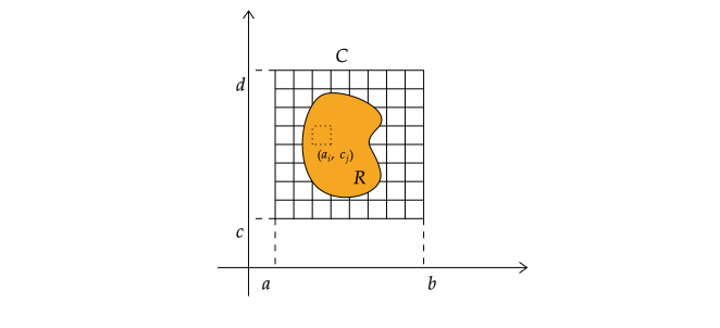 Every subbox of \(C\) meeting \(\bar{R}\) maps to a small patch of the surface. Let \(\{ a_{0}<a_{1}< \dots < a_{m}\}\) be a partition of \([a,b]\) and \(\{ c_{0} < c_{1} < \dots < c_{m} \}\) a partition of \([c,d]\). For \((a_{i},c_{j}) \in R\), define the curves \(\sigma_{a_{i}}:[c,d]\to S\) and \(\sigma_{c_{i}}:[a,b]\to S\) with \(\sigma_{a_{i}}(v) = \sigma(a_{i},v)\) and \(\sigma_{c_{i}}(u) = \sigma(u,c_{i})\). These curves have tangents
If we consider the subbox with corners \((a_{i},c_{j})\), \((a_{i+1},c_{j})\), \((a_{i},c_{j+1})\),\((a_{i+1},c_{j+1})\), then the area of the surface can be approximated by the area of the parallelogram formed by the tangent plane:
\[\begin{aligned} A_{S} &\approx \lVert (\sigma(a_{i+1},c_{j}) - (\sigma(a_{i},c_{j})) \times ((\sigma(a_{i},c_{j+1}) - \sigma(a_{i}, c_{j})) \rVert \\ &=_{TVM} \left\lVert (a_{i+1}-a_{i}) \frac{ \partial \sigma }{ \partial u }(u_{i},c_{j})\times (c_{j+1} - c_{j}) \frac{ \partial \sigma }{ \partial v }(a_{i},v_{j}) \right\rVert \\ &= (a_{i+1} - a_{i})(c_{j+1}-c_{j}) \left\lVert \frac{ \partial \sigma }{ \partial u }(u_{i},c_{j}) \times\frac{ \partial \sigma }{ \partial v }(a_{i},v_{j}) \right\rVert \end{aligned}\]with \(u_{i} \in [a_{i},a_{i+1}], v_{j} \in [c_{j},c_{j+1}]\). Summing over the subboxes and taking the limit as \(m \to \infty\):
\[\begin{aligned} \implies A_{S} &\approx \sum_{i,j=1}^{m} \underbrace{ (a_{i+1}-a_{i})(c_{j+1}-c_{j}) }_{ v(C) } \left\lVert \frac{ \partial \sigma }{ \partial u }(u_{i},c_{j}) \times\frac{ \partial \sigma }{ \partial v }(a_{i},v_{j}) \right\rVert \\ &\underset{m \rightarrow \infty}{\longrightarrow} \iint_{R} \left\lVert \frac{ \partial \sigma }{ \partial u }(u,v) \times\frac{ \partial \sigma }{ \partial v }(u,v) \right\rVert \, du \,dv = \iint_{R} \lVert N_{\sigma}(u,v) \rVert \, du \, dv. \end{aligned}\]Definition (Surface integral)
Given a continuous \(g:S\to R\), with \(S\) a surface, the surface integral is defined as
\[\iint_{S} g \, dS := \iint_{R} g(\sigma(u,v)) \lVert N_{\sigma} (u,v) \rVert \, du \, dv.\]Note that if \(g \equiv 1\), then \(\iint_{S} dS = \iint_{R} \lVert N_{\sigma}(u,v) \rVert \,du \,dv\) gives the area of \(S\).
Example (Sphere of radius 1)
In spherical coordinates we have \(\rho=1\). The parametrisation is given by: \(\sigma(\theta, \phi) = (\sin \phi \cos \theta, \sin \phi \sin \theta, \cos \phi)\), with \(\theta \in [0,2\pi], \phi \in [0,\pi]\).
- To compute the area, we obtain the normal vector:
So
\[A = \int_{0}^{2 \pi} \int_{0}^{\pi} \lvert \sin \phi \rvert \, d\phi \, d \theta = \int_{0}^{2\pi} \, d \theta \int_{0}^{\pi } \sin \phi \, d \phi = 4 \pi.\]- Let us now compute the tangent plane at \((\theta, \phi) = (\frac{\pi}{4}, \frac{\pi}{2})\). We first obtain a point of the plane by evaluating the surface at the given point:
Now we obtain the normal vector
\[N = -\sin \frac{\pi}{2} \left( \frac{\sqrt{ 2 }}{2}, \frac{\sqrt{ 2 }}{2},0 \right) =\left( \frac{-\sqrt{ 2 }}{2}, \frac{-\sqrt{ 2 }}{2}, 0\right).\]Hence the tangent plane is
\[\Pi: \left( \frac{-\sqrt{ 2 }}{2}, \frac{-\sqrt{ 2 }}{2},0 \right) \cdot \left( x - \frac{\sqrt{ 2 }}{2}, y - \frac{\sqrt{ 2 }}{2}, z\right) = 0.\]See more examples in the class notes
Oriented surfaces
Example
See the Möbius strip example.
Definition (Orientable surface)
- A unit normal vector for \(S\) at \((x_{0},y_{0},z_{0}) = \sigma(u_{0},v_{0})\)
- \(S\) is orientable if it has a \((\sigma, R)\) such that whenever \(\sigma (u_{0},v_{0}) = \sigma(u_{1},v_{1})\), then \(n_{\sigma}(u_{0},v_{0}) = n_{\sigma}(u_{1},v_{1})\).
-
Definition (Oriented surface integral)
Let \(S\) be an oriented surface with parametrisation \((\sigma, R)\) of class \(C^{1}\) and unit normal vector \(n\). Let \(F:S\to \mathbb{R}^{3}\) be continuous. We define
Note
Given \((\sigma_{1}, R_{1}), (\sigma_{2}, R_{2})\) for \(S\), then
\[\iint_{R_{1}} F(\sigma_{1}(u,v)) N_{\sigma_{1}} (u,v) \, du \, dv = \pm \iint_{R_{2}} F(\sigma_{2}(u,v)) N_{\sigma_{2}} (u,v) \, du \, dv.\]See examples in the class notes
The theorems of Green, Gauss and Stokes
Definition (Positive orientation for curves)
Let \(R \subseteq \mathbb{R}^{2}\) be a region with \(\partial R\) piecewise smooth. We say that \(\partial R\) has positive orientation if it carries the orientation induced by regarding \(R\) as a surface in \(\mathbb{R}^{3}\) (\(S =\{(x,y,0), (x,y) \in \mathbb{R}\}\)) with positive orientation (normal parallel to the \(z^{+}\) axis).
Theorem (Green)
Let \(R \subseteq \mathbb{R}^{2}\) be a region (as in the definition). Let \(F = (F_{1}, F_{2}):\mathbb{R}^{2} \to \mathbb{R}^{2}\) be of class \(C_{1}\). Then
\[\int_{\partial R} F \cdot T \, dS = \iint_{R} \left( \frac{ \partial F_{2} }{ \partial x } -\frac{ \partial F_{1} }{ \partial y }\right) \, dy \, dx .\]See examples in the class notes
Definition (Positive orientation for surfaces, and divergence)
- Let \(R \subseteq \mathbb{R}^{3}\) be a region with \(\partial R = S\) orientable and piecewise smooth. S is positively oriented if its unit normal vector \(n(x)\) points away from the interior \(R^{\circ}\) for every \(x\).
- Given \(F=(F_{1},F_{2},F_{3}):\mathbb{R}^{3}-.\mathbb{R}^{3}\) of class \(C^{1}\), its divergence is
Theorem (Gauss)
Let \(R \subseteq \mathbb{R}^{3}\) be a positively oriented region. If \(F:\mathbb{R}^{3} \to \mathbb{R}^{3}\) is of class \(C^{1}\), then
\[\iint_{\partial R} F \cdot n \, dS = \iiint_{R} \mathrm{div} F \, dz \,dy \,dx\]See examples in the class notes
Definition (Curl)
Given \(F:\mathbb{R}^{3}\to \mathbb{R}^{3}\) of class \(C^{1}\), its curl is defined as
\[\mathrm{rot F} = \nabla \times F = \begin{vmatrix} \hat{i} & \hat{j} & \hat{k} \\ \frac{ \partial }{ \partial x } & \frac{ \partial }{ \partial y } & \frac{ \partial }{ \partial z } \\ F_{1} & F_{2} & F_{3} \end{vmatrix} = \left( \frac{ \partial F_{3} }{ \partial y } - \frac{ \partial F_{2} }{ \partial z }, -\frac{ \partial F_{3}}{ \partial x } + \frac{ \partial F_{1} }{ \partial z }, \frac{ \partial F_{2} }{ \partial x } - \frac{ \partial F_{1} }{ \partial y } \right)\]Theorem (Stokes)
Let \(S\) be an orientable surface of class \(C^{2}\), piecewise smooth, with normal \(n\). Suppose that “\(\partial S\)” is a closed curve of class \(C^{1}\), piecewise smooth and positively oriented. If \(F:\mathbb{R}^{3}\to \mathbb{R}^{3}\) is of class \(C^{1}\), then
\[\iint_{\partial S} F \cdot T \, dS = \iint_{S} \mathrm{rot} F \cdot n \, dS.\]Note
Here the “boundary of \(S\)” does not refer to its topological boundary (since every point satisfies that definition). We mean instead the image of \(\partial R\), where \(S = (\sigma, R)\).
See examples in the class notes